

E3SMv2 Performance Highlighted at AGU Session

E3SM v2 performance improvements were recently highlighted at the AGU Fall Meeting, which took place from 13 to 17 December 2021 as a hybrid conference with both online participants and in-person attendees in New Orleans.
High Performance Computing session on Earth System Modeling
Sarat Sreepathi (Primary Convener) and Phil Jones (Session Chair) of the E3SM Performance group along with collaborators organized a High Performance Computing (HPC) session focused on Earth System Modeling.
In conjunction with related Artificial Intelligence submissions, the combined thematic session named “Accelerating Earth System Predictability: Advances in High Performance Computing, Numerical modeling, Artificial Intelligence and Machine Learning” had two oral components (Session I and Session II) and related posters (eLightning and poster sessions). This session attracted a diversity of submissions in topic breadth as well as geographical representation resulting in a total of fifteen talks and sixteen poster presentations.

Figure 1. Cloud distribution simulated by the NICAM 870 m grid spacing experiment for 6:00 UTC 25 August 2012 (Miyamoto et al. [2013] ).
Within the HPC focused oral session, there were two invited talks. Chihiro Kodama from JAMSTEC/Japan presented their recent progress on developing NICAM (Nonhydrostatic Atmospheric ICosahedral Model, Fig.1) on the Japanese supercomputer Fugaku with an eye towards realization of a global cloud-resolving (3.5 km mesh) climate simulation. Kim Serradell from the Barcelona Supercomputing Center detailed their efforts on collecting computational performance data from various Earth System Models participating in the Coupled Model Intercomparison Project (CMIP) within the framework of the IS-ENES3 project (European Network for Earth System Modelling).
Additionally, there were a diversity of talks including a discussion of nesting capability of the GFDL’s Finite-Volume Cubed-Sphere Dynamical Core (FV3) and a couple of talks describing ocean model developments using Julia and Python programming languages promising performance and productivity gains.
E3SM and related ecosystem projects had a strong representation with an oral presentation by Andrew Bradley on algorithmic and performance improvements in E3SMv2 Atmosphere Model (EAM, Fig. 2), two eLightning (Azamat Mametjanov on tuning E3SM performance on Chrysalis, Thomas Clevenger on performance of Simple Cloud Resolving E3SM Atmosphere Model (SCREAM)) and three poster presentations (Rong-You Chien on high-efficiency chemistry solver, Matt Norman on performance portability efforts within E3SM-MMF, and Xingqiu Yuan on performance comparison of different programming models).
Algorithmic and Performance Improvements in E3SMv2
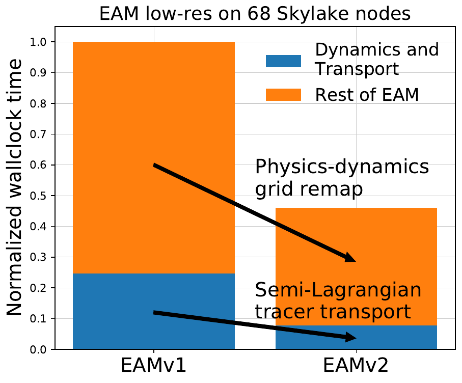
Figure 2. Normalized wallclock time of the E3SM Atmosphere Model (EAM) versions 1 and 2. Two new algorithms in EAM version 2 make it approximately twice as fast as EAM version 1 (Bradley, AGU 2021). First, physics parameterizations are run on a new physics grid having 4/9 as many columns as in version 1; new algorithms remap data between the dynamics and physics grids (the speedup in the orange blocks). Second, semi-Lagrangian tracer transport speeds up the dynamical core by approximately three times (the blue blocks).
Andrew Bradley presented the perfomance improvements of E3SMv2 over E3SMv1. Two new methods in the E3SM Atmosphere Model version 2 (EAMv2) increase the computational efficiency of EAM by a factor of approximately two in multiple configurations and on multiple platforms. EAM consists of the High-Order Methods Modeling Environment (HOMME) Spectral Element (SE) dynamical core (dycore) and the EAM physics and chemistry parameterizations. The most expensive parts of EAM are tracer transport in the dycore and parameterizations (Fig. 2). Two related methods speed up each of these: high-order, property-preserving, remap-form, semi-Lagrangian tracer transport (SL transport) and high-order, property-preserving physics-dynamics-grid remap (physgrid remap). SL transport replaces the dycore’s Eulerian flux-form method, enabling much greater simulation time per computational communication round. Physgrid remap enables running parameterizations on a grid that approximately matches the effective resolution of the SE dycore. This procedure replaces running parameterizations on the denser dynamics grid.
Figure 3 shows details of EAM performance on the ANL LCRC Chrysalis system, expanding on the results in Figure 2. The tracer transport curves in (a) and the red regions in (b) show that tracer transport is 6 to over 8 times faster in v2 than v1. The “Total” curves in (a) and the total normalized time in (b) show that EAMv2 is over 2 and up to 2.5 times faster than EAMv1.
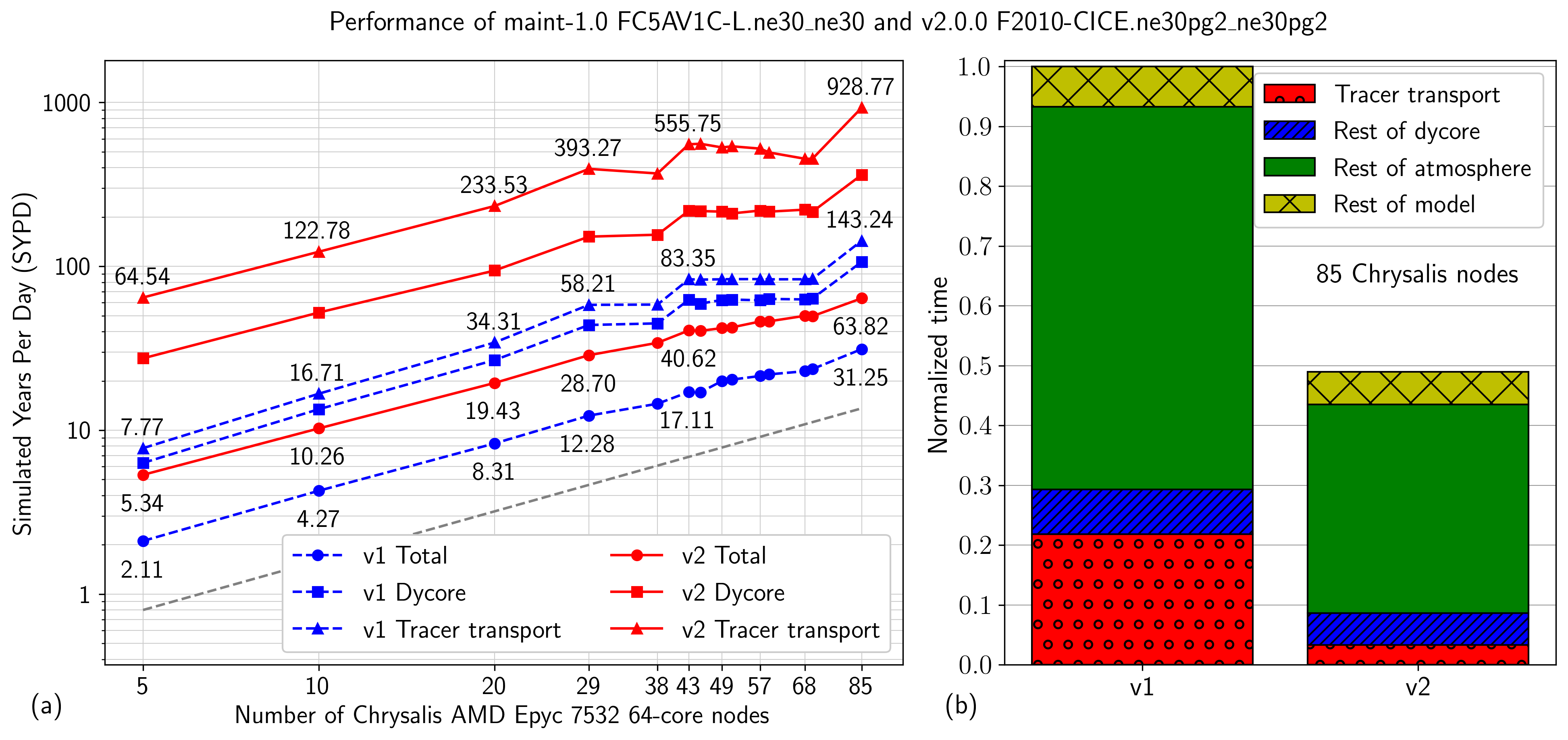
Figure 3. Performance of the low-resolution EAMv1 and EAMv2 atmosphere simulations on the ANL LCRC Chrysalis system (Bradley, AGU 2021). (a) Throughput in Simulated Years Per Day (SYPD) vs. number of Chrysalis nodes. Annotations of individual data points are SYPD values. Throughput is shown for tracer transport, the dynamical core as a whole (“Dycore”), and EAM as a whole (“Total”). (b) Proportion of time spent in each subcomponent in the 85-node case, with the total time for v1 normalized to 1 as in Figure 2.
Figure 4 shows performance of the Water Cycle preindustrial control, low-resolution, fully coupled simulations for XS, S, M and L model configuration on PE nodes, again on Chrysalis (see the caption for details). In this configuration, the atmosphere and land share a cubed-sphere grid having 30-by-30-element faces, for approximately 110km atmosphere dynamics grid resolution and 165km atmosphere physics and land grid resolution in v2, and 110km resolution for all of these in v1. The ocean and sea ice share a grid having cells of 30 to 60km diameter. Comparing S, M, and L layouts between models, v2 is at least 1.97 times more efficient than v1. Figure 4(b) illustrates this efficiency difference by plotting the throughput-resource product for each component as a rectangle for the L layouts. The atmosphere (ATM), sea ice (ICE), coupler (CPL), land (LND), and river runoff (ROF; LND and ROF are too small to label) components run on one set of nodes, while the ocean (OCN) component runs on another set. An unfilled rectangle having v1 or v2 at the top-right corner shows the total product; because the throughput value of each component is approximate, the filled rectangles do not sum to the total throughput value. As in Figure 3, the atmosphere component is over twice as efficient in v2 as in v1. MPAS-Ocean in v2 is approximately 2.8 times more efficient than in v1 because the ocean dynamics time step is three times larger in v2 than in v1. The MPAS-Seaice component is slower in v2 than in v1 because of additional snow layers.
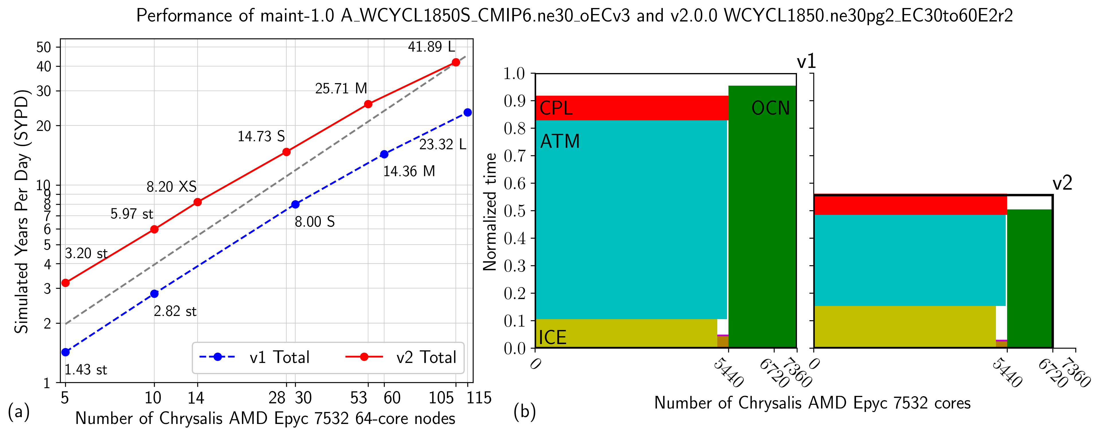
Figure 4. Performance of the low-resolution E3SMv1 and E3SMv2 preindustrial control simulations (Bradley, AGU 2021). (a) Throughput vs. number of nodes. Annotations of individual data points are SYPD values and PE layout. The PE layout is the configuration of the model on the nodes. PE layouts XS, S, M, L are provided as part of the models. Points annotated with “st” use a simple stacked layout in which each component runs serially with respect to the others, and all components share the same processors. (b) Throughput-resource-product plots. Each component has one rectangle. A rectangle is the area given by the product of throughput and number of nodes.
The two new EAM methods work seamlessly both in the standard EAM configuration and in the Regionally Refined Mesh (RRM) configuration. The E3SMv2 low-resolution and RRM coupled configurations use these features. On E3SM’s ANL LCRC Chrysalis system, based on AMD Epyc 7532 processors, the low-resolution coupled model achieves over 41 simulated years per day (SYPD) on 105 nodes (Fig. 4), and the North America RRM coupled model achieves over 12 SYPD on 100 nodes. This improved computational performance enables researchers to run longer simulations to address scientific questions previously not feasible.
Related Articles
This article is a part of the E3SM “Floating Points” Newsletter, to read the full Newsletter check: