

v2 NARRM Description
The Energy Exascale Earth System Model version 2.0 (E3SMv2) release supports two horizontal resolutions. The standard low-resolution (LR) version (i.e., 110 km atmosphere, 165 km land, 55 km (at the equator) river, and 30km-60km ocean and sea ice) was highlighted in an earlier newsletter article “E3SMv2 overview paper“. Unlike the E3SMv1 high-resolution version, which uses the global uniform grids, the E3SMv2 high-resolution version adopts the regionally refined mesh in all components (except river). This makes the E3SMv2 North American (NA) Regionally Refined Model (NARRM) the first Earth system model with fully coupled RRM which successfully delivered the climate production simulations, e.g., the Coupled Model Intercomparison Project 6 (CMIP6) DECK (Diagnosis, Evaluation, and Characterization of Klima) and historical simulations.
Key points
- The NARRM makes E3SM the first-of-its-kind, global fully coupled model with RRM implemented in all components (except river), that completed climate production simulations.
- The NARRM has great computational efficiency (~10-20%) relative to a global uniform high-resolution model.
- The global climate, including climatology, time series, sensitivity, and feedback, is confirmed to be largely identical between NARRM and the low-resolution (LR) E3SMv2 configurations.
- Over the refined area, NARRM is generally superior to LR, including for precipitation and clouds over the contiguous US (CONUS), summertime marine stratocumulus clouds off the coast of California, liquid and ice phase clouds near the North Pole region, extratropical cyclones, and spatial variability in land hydrological processes.
The NARRM is developed with the primary goal of more explicitly addressing DOE’s mission needs regarding impacts to the US energy sector facing Earth system changes, and hence the finer resolution grids centered over NA (see Fig. 1, 25→100 km atmosphere and land, a 14 km (at the equator) river-routing model, and 14→60 km ocean and sea ice). By design, the computational cost of E3SMv2 NARRM is only ~10-20% of a globally uniform high-resolution model at 25 km. It is worth noting that E3SM RRM model is highly configurable and the refinement can be set up over any region of the globe and can be any size.
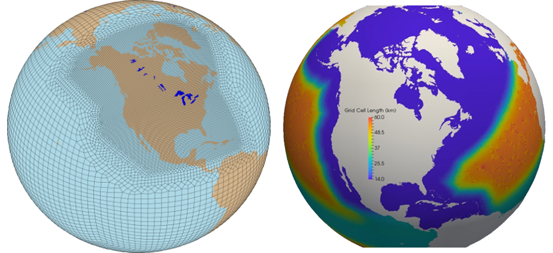
Figure 1. North American RRM (NARRM) grids for the atmosphere and land (left, 25->100km) and for the ocean and sea ice (right, 14->60km) (Need to rearrange the two panels.)
Thanks to the novel hybrid time step strategy in the atmospheric model, the NARRM achieved improved climate simulation fidelity within the high-resolution patch without sacrificing the overall global performance. The hybrid time step method combines the high-resolution time step for dynamics and the low-resolution time step for physics. This is a practical choice due to the poor scale-aware atmospheric physics (i.e., the deep convection scheme and other cloud parameterizations). The outcome is that NARRM is able to retain much of the low-resolution global climate features with some improvements from the high-resolution dynamics. Another benefit of the hybrid time step approach is that it minimizes the retuning effort beyond the low-resolution configuration.
Global Climatology
For the global climatology, Figure 2 focuses on years 1985-2014, the last portion of historical simulations when more observational data are available. It shows that NARRM and LR models are generally very similar as measured by the spatial root-mean-square error (RMSE) of important variables relative to the observations or reanalysis datasets. Smaller RMSE values mean better performance. For example, NARRM simulates slightly better clouds and precipitation, and slightly worse zonal wind for some seasons.
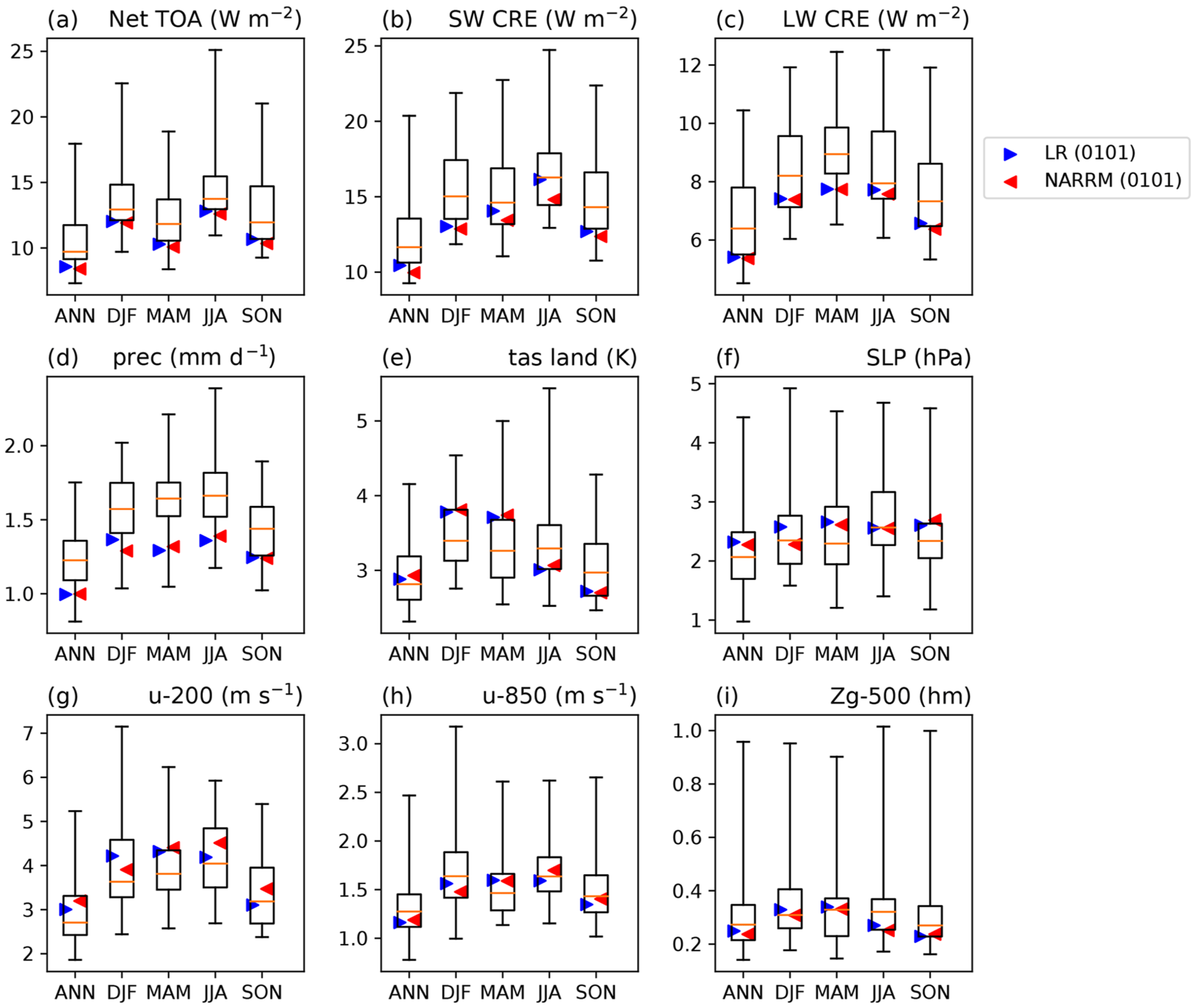
Figure 2. Comparison of the global spatial RMSE of model climatology (annual and seasonal averages of years 1985–2014) vs. observations. The model results are from the first historical member of E3SMv2 (0101), LR (blue triangles), and NARRM (red triangles) and 52 CMIP6 models (r1i1p1f1). The boxes and whiskers show the 25th percentile, 75th percentile, and minimum and maximum RMSE of the CMIP6 ensemble. Quantities include (a) TOA net radiation flux, (b, c) TOA SW and LW cloud radiative effects, (d) precipitation, (e) surface air temperature over land, (f) sea level pressure, (g, h) 200 and 850 hPa zonal wind, and (i) 500 hPa geopotential height. TOA is the top of the atmosphere, SW is shortwave, CRE is cloud radiative effects, LW is longwave, ANN is annual, DJF is December–February, MAM is March–April, JJA is June–August, SON is September–November, and RMSE is root-mean-square error.
Climate Sensitivity
The NARRM also mimics the LR characteristics in terms of the climate sensitivity and feedback. Figure 3 illustrates the equilibrium climate sensitivity (ECS), the transient climate response (TCR), and the 2xCO2 effective radiative forcing (ERF) from NARRM and LR derived from the idealized CO2 experiments. The differences in all these quantities between NARRM and LR are very subtle.
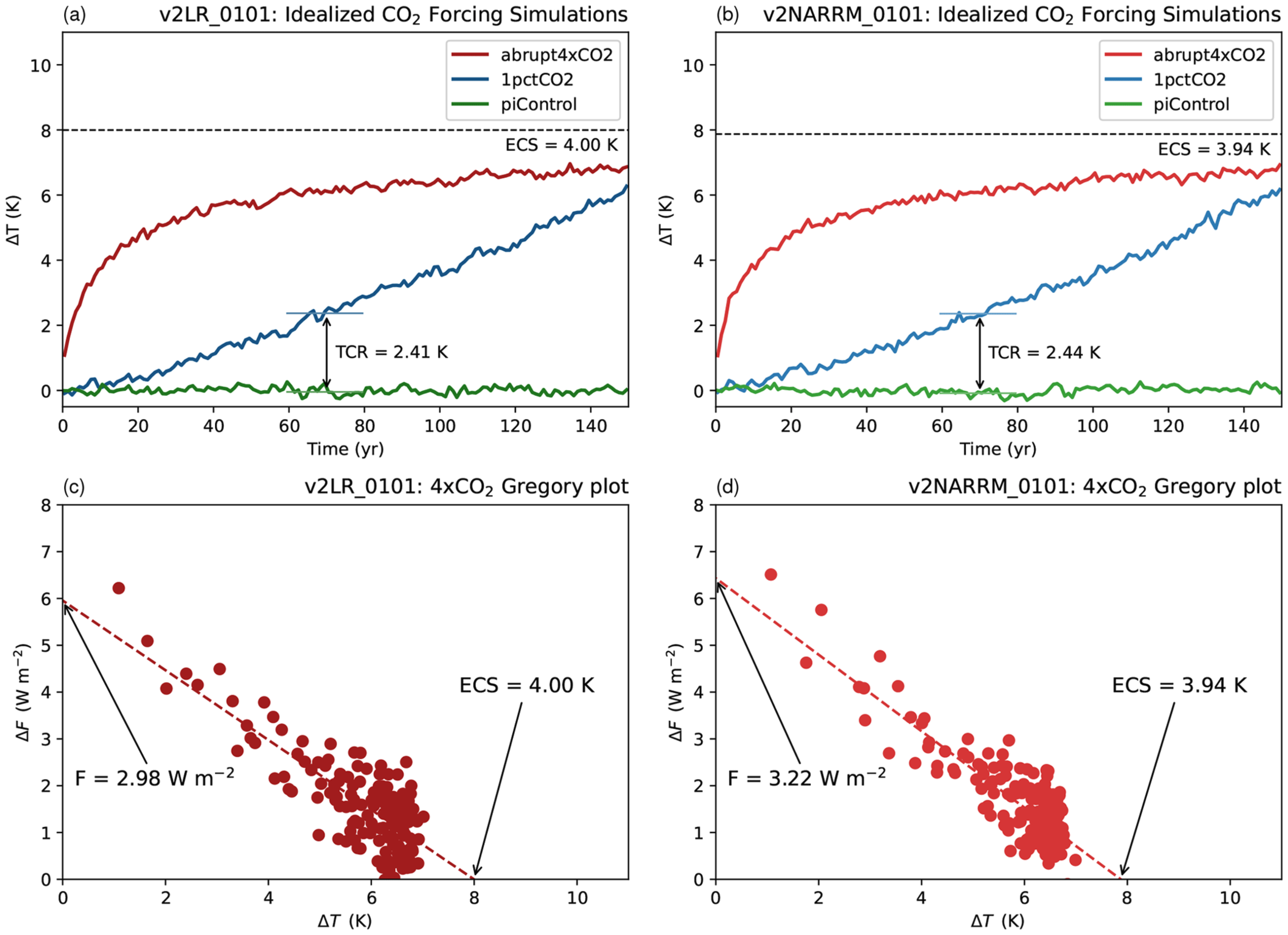
Figure 3. Comparison of climate sensitivities between LR (a, c) and NARRM (b, c) derived from idealized CO2 forcing simulations. (a, b) time series of global annual mean surface air temperature anomaly from the following simulations, abrupt-4xCO2 (red), 1pctCO2 (blue), and the control (piControl; green). The transient climate response (TCR) is computed as a 20-year average around the time of CO2 doubling (year 70). (c, d) Gregory regression plots (Gregory et al., 2004). The estimated effective climate sensitivity (ECS) and effective 2× CO2 radiative forcing (F) are as labeled.
North American (NA) Region
When zooming in over the refined NA region, NARRM demonstrates several great improvements compared to LR, including some long-standing problems (e.g., marine stratocumulus clouds and mixed-phase clouds) that plague many Earth system models. Figure 4 shows that the underestimation of summertime low clouds (manifested as the excessive (red) top of atmosphere (TOA) shortwave cloud radiative effect CRE) in the California stratocumulus region is substantially improved with NARRM. This improvement is likely due to a reduced bias in the simulated sea surface temperature (SST) in the coupled RRM and highlights the advantage of coupled RRM over a single-component RRM.
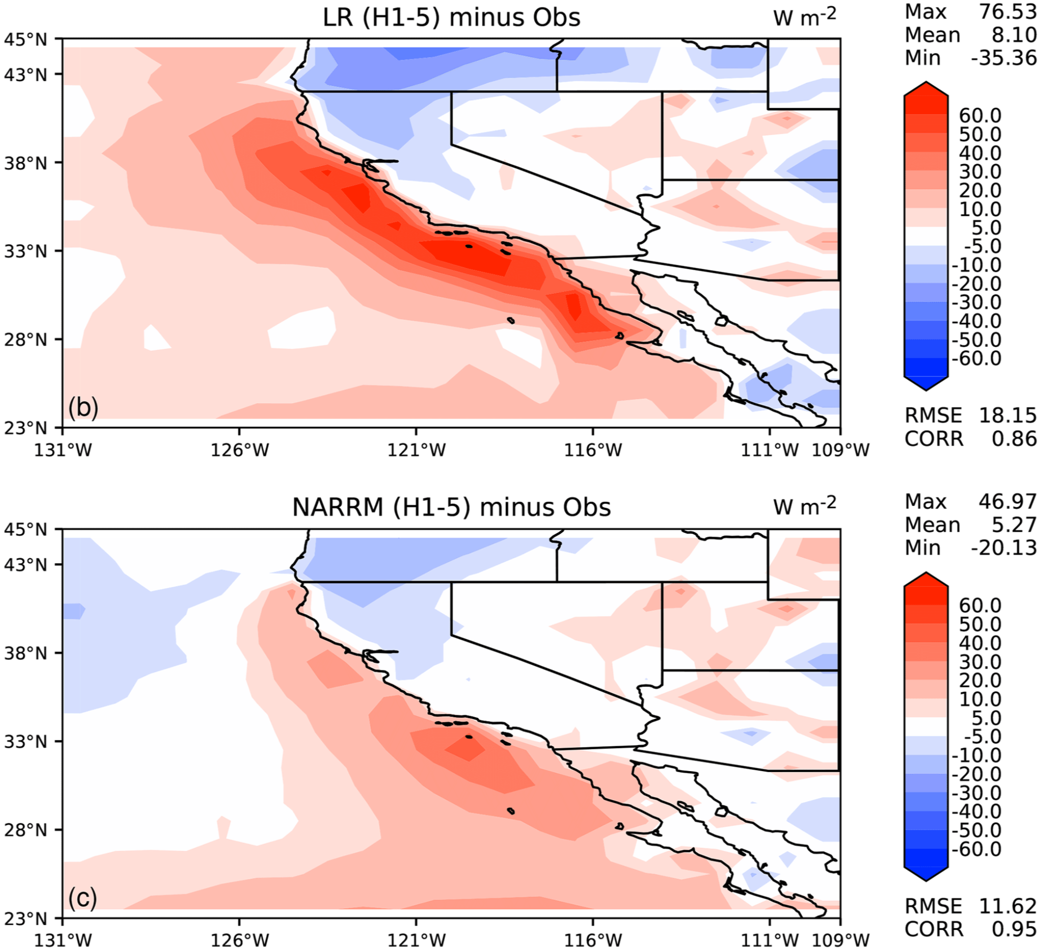
Figure 4. Mean TOA shortwave cloud radiative effects at California in JJA of (top) LR (H1-5) minus observation, and (bottom) NARRM (H1-5) minus observation.
Another example is the mixed-phase clouds near the Arctic. It has been a challenge to simultaneously improve the simulation of liquid and ice clouds there with atmosphere-only simulations. The coupled NARRM displays improved annual mean cloud cover in both liquid and ice phases relative to LR (see Fig. 5). These NARRM improvements are due to the better represented topography over land and the more realistic air-sea interactions over ocean.
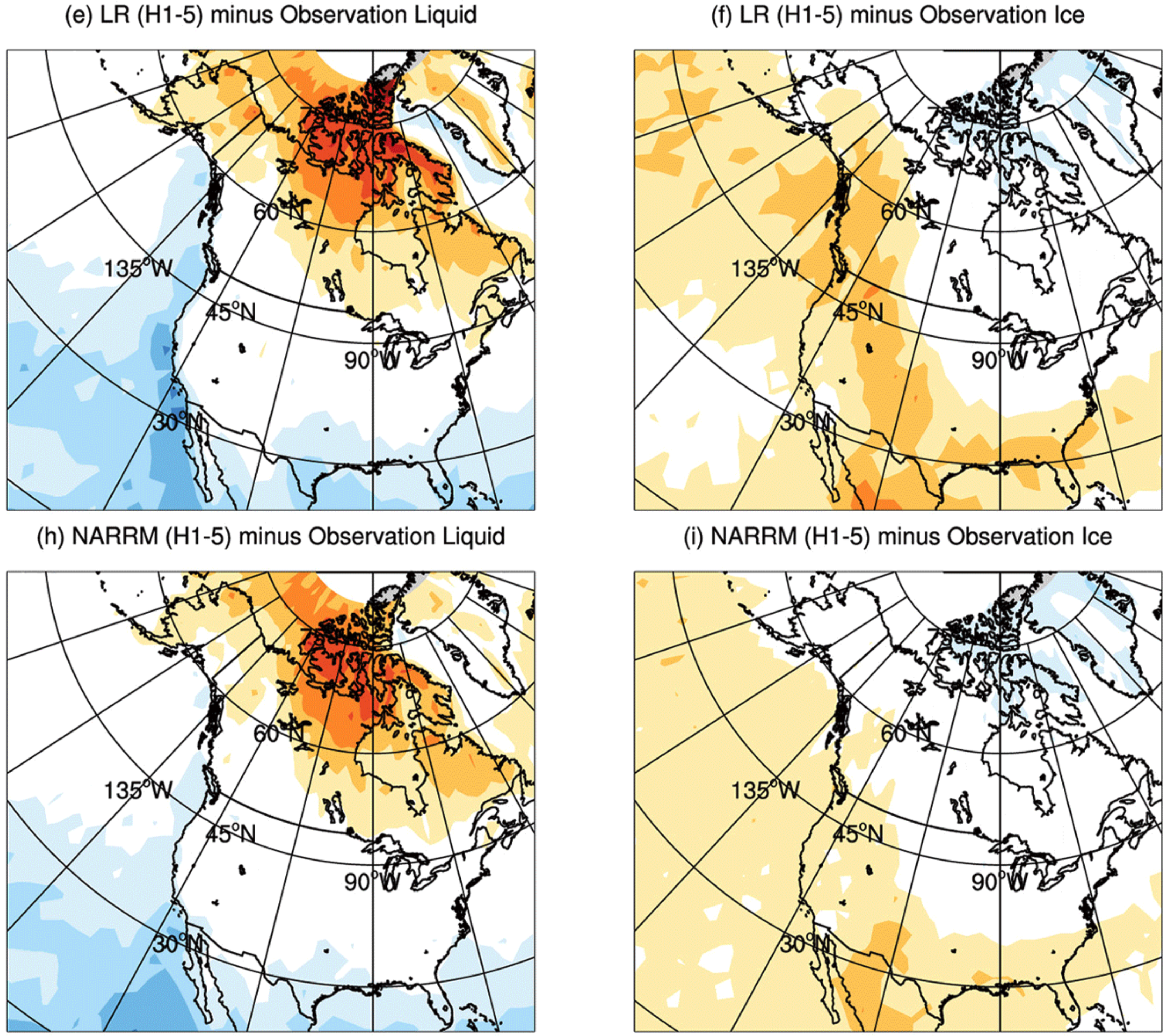
Figure 5. Spatial distribution of annual mean cloud cover biases relative to the CALIPSO-GOCCP observations in (left) liquid phase and (right) ice phase for (top) LR (H1-5) and (bottom) NARRM (H1-5) historical simulations (1985–2014).
Besides all these improvements, the NARRM configuration has some weaknesses. A major one is that the hybrid time step strategy, as a practical choice, cannot take full advantage of the resolved processes (e.g., updrafts) with the high-resolution dynamics because of the large time-truncation errors. We are testing alternative approaches to overcome this weakness when developing the next release of NARRM. Our initial tests show encouraging results and we will report more about our RRM advances in future news.
Code and Data Availability
The E3SM code used in this work is available at https://doi.org/10.5281/zenodo.7343230 and on GitHub at https://github.com/E3SM-Project/E3SM, including a maintenance branch (maint-2.0; https://github.com/E3SM-Project/E3SM/tree/maint-2.0) that has been created to reproduce these simulations.
The complete native model output and the nudging simulations’ climatology data are accessible directly at the National Energy Research Scientific Computing Center (NERSC) (https://portal.nersc.gov/archive/home/projects/e3sm/www/WaterCycle/E3SMv2/LR, and https://portal.nersc.gov/archive/home/projects/e3sm/www/WaterCycle/E3SMv2/NARRM for low-resolution and NARRM simulations, which are documented at https://e3sm-project.github.io/e3sm_data_docs. A subset of the native output is also available through the DOE Earth System Grid Federation (ESGF) at https://esgf-node.llnl.gov/search/e3sm/?model_version=2_0. Data reformatted following CMIP conventions will also be available through ESGF at https://esgf-node.llnl.gov/projects/e3sm.
Performance data and scripts are located at https://github.com/E3SM-Project/perf-data/tree/archive/v2-narrm-perf-study/v2-narrm and https://doi.org/10.5281/zenodo.8114977.
Reference
- Tang, Q., Golaz, J.-C., Van Roekel, L. P., Taylor, M. A., Lin, W., Hillman, B. R., Ullrich, P. A., Bradley, A. M., Guba, O., Wolfe, J. D., Zhou, T., Zhang, K., Zheng, X., Zhang, Y., Zhang, M., Wu, M., Wang, H., Tao, C., Singh, B., Rhoades, A. M., Qin, Y., Li, H.-Y., Feng, Y., Zhang, Y., Zhang, C., Zender, C. S., Xie, S., Roesler, E. L., Roberts, A. F., Mametjanov, A., Maltrud, M. E., Keen, N. D., Jacob, R. L., Jablonowski, C., Hughes, O. K., Forsyth, R. M., Di Vittorio, A. V., Caldwell, P. M., Bisht, G., McCoy, R. B., Leung, L. R., and Bader, D. C.: The fully coupled regionally refined model of E3SM version 2: overview of the atmosphere, land, and river results, Geosci. Model Dev., 16, 3953–3995, https://doi.org/10.5194/gmd-16-3953-2023, 2023.