

Islet: Interpolation Semi-Lagrangian Element-Based Transport
The Science
Advection of trace species, or tracers, in models of the atmosphere and other physical domains is an important and computationally expensive part of a model’s dynamical core. Tracers are used in models of atmospheric microphysics and macrophysics, convection, aerosols, and chemistry. Atmosphere models may use from tens to hundreds of tracers. Thus, it is important that tracer transport be computed extremely efficiently.
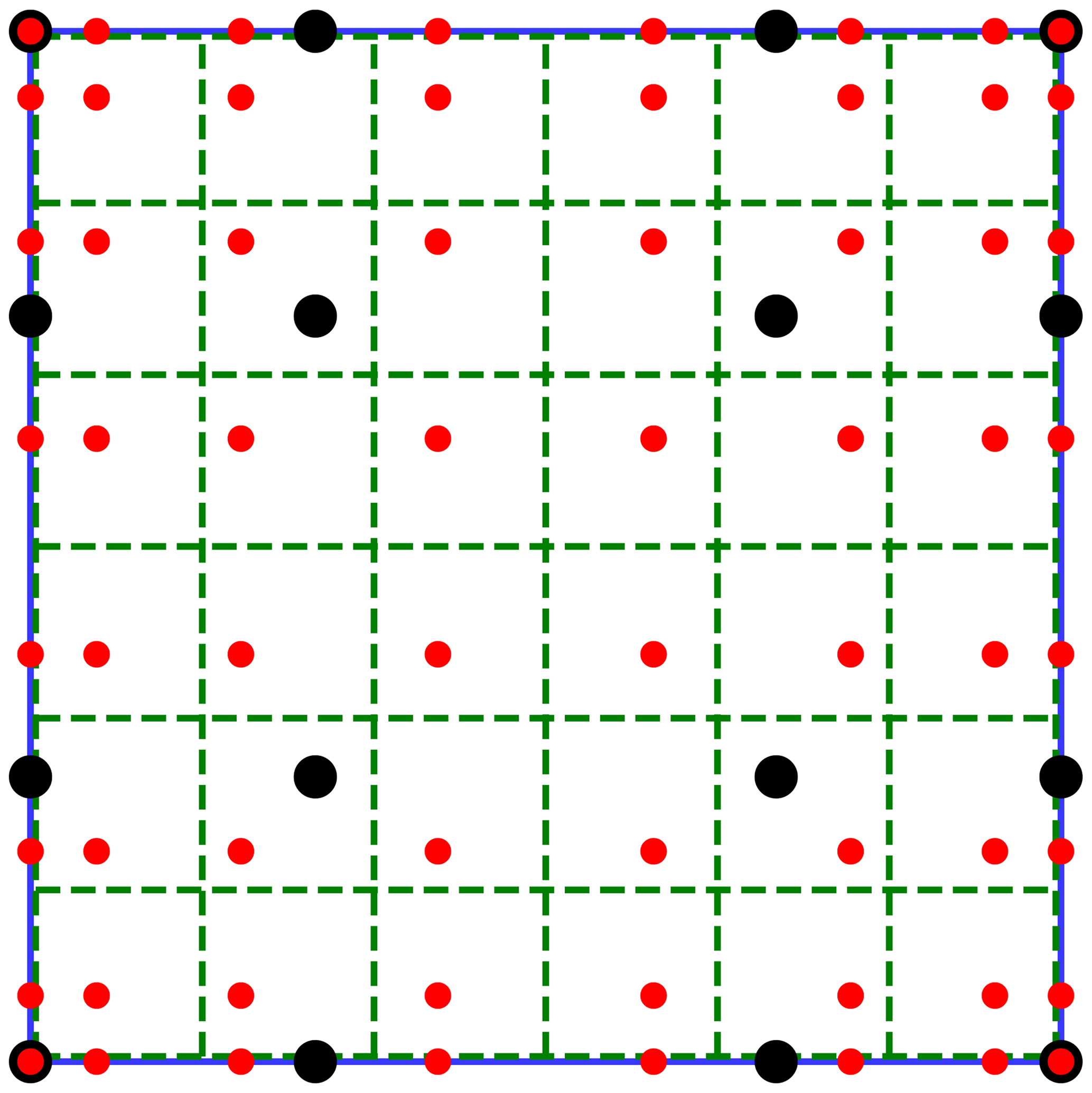
Figure 1. Diagram of subelement grids. One spectral element (blue solid line outlining the full square) with dynamics (np_v=4, black large circles), tracer (np_t=8, small red circles), and physics (n_f=6, green dashed lines) subelement grids.
In general, advection of trace species in models of the atmosphere is a computationally expensive part of a model’s dynamical core. To solve the tracer transport problem, one can use Lagrangian or Eulerian methods, or their combination. In a Lagrangian method, the model grid is distorted to follow the flow, and material follows the grid. In an Eulerian method, the grid is fixed and material flows across the grid. In a Semi-Lagrangian (SL) method, material is remapped between the flow-distorted grid and the background Eulerian grid at each time step. Semi-Lagrangian advection methods are efficient because they permit a time step much larger than the advective stability limit for explicit Eulerian methods without requiring the solution of a globally coupled system of equations as implicit Eulerian methods do. Thus, to reduce the computational expense of tracer transport, dynamical cores often use SL methods to advect tracers. Among SL methods, the interpolation semi-Lagrangian (ISL) methods are particularly efficient, and this study developed an ISL method suited to spectral element grids.
The Impact
The scientists developed a method called the Interpolation Semi-Lagrangian Element-based Transport (Islet) method for use in the E3SM Atmosphere Model. The Islet method uses three grids: a dynamics grid, a physics parameterizations grid, and a tracer grid supporting the use of the new Islet basis functions. Each grid’s subelement structure is independently configurable (Fig. 1). These separate grids permit the dynamics, tracer transport, and physics parameterizations of each to be as efficient as possible, leading to an overall atmosphere simulation that is extremely efficient. The lowest-order Islet transport method is used in the E3SM Atmosphere Model version 2. It speeds up atmosphere tracer transport over version 1 by a factor of six to eight and provides a slightly higher resolution. Higher-order variants could be used to better resolve and maintain filamentary structures in tracers while using the same dynamics and physics parameterizations configurations, as shown in the bottom three rows of Figure 2.
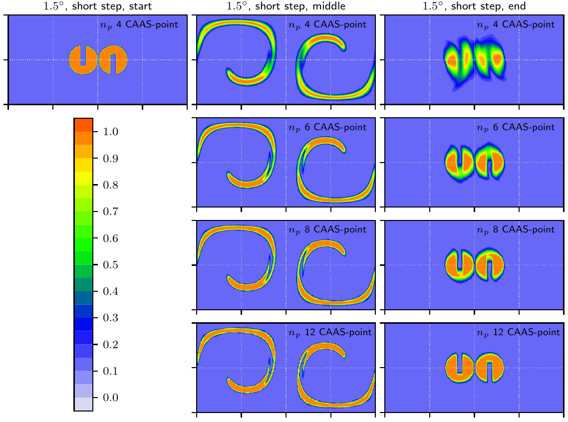
Figure 2. Example of tracer transport at multiple resolutions. The velocity data (representing the dynamics) and time steps are the same in each case. Time proceeds left to right. Resolution increases top to bottom. The exact solution at the final time (right column) is the same as the initial condition (left column).
Summary
The scientists developed the finite-element ISL transport Islet method for use with atmosphere models discretized using the spectral element method, including the E3SM Atmosphere Model (EAM). The Islet method uses three independently configurable grids that share an element grid: a dynamics grid supporting, for example, the Gauss-Legendre-Lobatto basis of degree three (Dennis et al., 2005), as is standard in EAM; a physics parameterizations grid with a configurable number of finite-volume subcells per element; and a tracer grid supporting the use of Islet bases, with the particular basis again configurable. The Islet method provides remap operators to transfer data among these three grids for use in time stepping. Putting these pieces together, the Islet method yields extremely accurate tracer transport and excellent diagnostic values for a number of verification problems.
Figure 2 shows an example of the Islet method applied to a standard test problem. Time proceeds left to right. Tracer grid basis order of accuracy increases from top to bottom. The velocity data and time steps are the same across rows. Images are shown on the dynamics grid, not the higher-resolution tracer grids. The exact solution is the same as the initial condition (top-left panel). The initial condition is discontinuous, the hardest case for high-order methods. Nonetheless, as the Islet basis increases in order of accuracy, with all other parameters held fixed, the solution accuracy (right column) increases substantially and filaments are resolved more accurately (middle column).
The new tracer transport method is used in EAM version 2, and is 6.5 to over 8 times faster than in EAM version 1 in the cases of, respectively, low and high workload per computer node (Golaz et al., 2022, Fig. 3). In addition, remap operators were developed to remap data between separate grids for physics parameterizations and dynamics, permitting the physics parameterization computations to run on a coarser grid and thus 1.6 to 2.2 times faster in version 2 than in version 1 (Hannah et al., 2021; Golaz et al., 2022).
Publication
- A. M. Bradley, P. A. Bosler, and O. Guba: Islet: interpolation semi-Lagrangian element-based transport, Geosci. Model Dev., 15, 2022, https://doi.org/10.5194/gmd-15-6285-2022.
Funding
- This work was supported by the US Department of Energy (DOE) Office of Science’s Advanced Scientific Computing Research (ASCR) and Biological and Environmental Research (BER) Programs under the Scientific Discovery through Advanced Computing (SciDAC 4) ASCR/BER Partnership Program.
Contact
- Andrew M. Bradley, Sandia National Laboratories
Related
This article is a part of the E3SM “Floating Points” Newsletter, to read the full Newsletter check: