Visualizing Earth’s Water Cycle through E3SM Simulations
Earth’s water cycle is a non-trivial multiscale system. Following water molecules along the circular conceptual path of evaporation, condensation, precipitation, and accumulation in an Earth system model requires multi-phase simulations in land, ice, ocean, and the atmosphere. Visualizing this flow and processing the data for scientific gain is uniquely challenging, and a multi-dimensional space (three spatial dimensions and the time component) is necessary to comprehend its grandeur.
Traditionally, components of the water cycle have been viewed in two-dimensional contour plots, with latitude and longitude or time and space axes. These types of visualizations are often used in journals and presentations. In the case of the water cycle, water flow through the system is often averaged across time or space dimensions. In this work, new ways have been explored to visualize the multiple components of the simulated Earth system by using tools capable of projecting time-evolving fluids on a spherical coordinate system. This new set of tools includes ParaView, Houdini, Unity, and the new Universal Scene Description (USD) data format. New hardware has also been tested, allowing users to experience Earth systems data in virtual reality. Two types of simulations were visualized. The first type was a coupled-model configuration in which all components of the Earth system from the Energy Exascale Earth System Model (E3SM) were active. The second type was an atmosphere-only model with a simplified representation of the cloud physics to simulate a supercell thunderstorm.
Care was taken throughout the visualization development to document workflows and use free versions of commercial-off-the-shelf and open-source tools. This was done so that the visualization products could be reproduced by new users as new features in the simulations are discovered.
Energy Exascale Earth System Model Water Cycle Campaign
E3SM is the Department of Energy’s (DOE) Earth system model designed to answer DOE science questions using DOE computing facilities. The E3SM project includes three sets of simulation experiments: cryosphere, bio-geochemical cycles, and the water cycle. The water cycle experiment campaign includes a set of simulations designed to understand how the water cycle will change in coming decades under a changing climate. The general circulation of the atmosphere, including precipitation from storm tracks and weather extremes, is the focus of this visualization activity because these Earth system elements are short-lived, but impactful events.
To generate this data, E3SM was run in its coupled high-resolution configuration with active land, atmosphere, ice, and ocean components on the Theta supercomputer using ~800 nodes. Data from the atmosphere was output every simulated hour, and data from the ocean output every day.
This high-resolution configuration of the coupled E3SM components has some of the highest spatial resolutions of any model in its class. However, the spatial resolution in the atmosphere – roughly 25 kilometers – is still not sufficient to resolve clouds and convection. A sub-cell, or sub-grid, parameterization is needed to provide the instability that creates storms. To probe the ability of a global climate model to run at even higher spatial resolutions than 25 kilometers in the atmosphere and resolve severe storms without the use of sub-grid parameterizations, the E3SM team has developed a version of the atmosphere designed to resolve large convective events. To test this capability, a configuration using simplified cloud physics and a fictional small planet with a radius 1/120th the size of the Earth was used, making the numerical simulation computationally feasible while providing enough detail to resolve a storm. The test case is a supercell thunderstorm. It appears enormous relative to the fictional planet since it covers roughly one-sixth of the available surface area. The simulation produced timesteps spaced at 15 second intervals, with the thunderstorm developing to full strength over two simulated hours.
Generation of Visualizations
Coupled simulation
Figure 1. Transition from an ocean-only visualization to the coupled atmosphere-ocean visualization. The ocean data has been interpolated linearly to hourly timesteps. In the final few frames, a cold water wake created by a storm can be seen. In the final version of this animation, the transition sequence will be longer. The landmasses are black, the ocean is visualized with warmer and cooler colored contours of sea-surface temperatures, and the atmosphere’s cloud fraction is in grey-scale.
Part of the tasking of this project was to create a visualization of the coupled water-cycle simulation; one of the major difficulties with visualizing this data is that each component of the dataset can be output at different timescales, ranging from hourly to monthly. In order to accommodate the range in output E3SM timescales, two design choices were made for creating the visualization: using SideFX’s Houdini software for rendering and animation, and Pixar’s USD for data interchange, since USD can represent all of the geometry types needed for the final visualization along with the multiple timescales required for the project. In addition, USD is actively supported by a majority of tools for digital content creation (DCC), including Maya, Houdini, and the Unity and Unreal game engines.
An important requirement was a workflow to convert E3SM data into the USD data format. Over the past year, researchers at Sandia have been developing expertise representing scientific data using USD. While typical workflows might use ParaView directly for visualization, in this case additional work was necessary to convert ParaView outputs to USD. A C++ tool was developed that could ingest most of the file formats exportable from ParaView (and by extension, VTK, the underlying framework for ParaView), so the resulting workflow was E3SM Data → ParaView → C++ tool → USD. In the future, given additional resources, it would be ideal to convert this tool to a ParaView plugin that could export the data to USD directly.
For the simulations, the ocean data is output on a two-dimensional, unstructured, time-varying mesh using daily timesteps, and the atmospheric data is output on a three-dimensional, unstructured, time-varying mesh using hourly timesteps. A series of ParaView batch scripts load and then export the E3SM data with a reduced set of variables into parallel ParaView unstructured data files. These files are then converted to the USD format and imported into Houdini for animation and rendering.
Following import the team explored how to handle the different timesteps for the different components. The default for USD is to hold a timestep of data across however many sub-timesteps are in the animation, until the next valid timestep for the data is reached. In the case of the E3SM data, the daily ocean data is held across the 24 sub-steps of the hourly atmospheric data. However, USD and Houdini provide the flexibility to interpolate the ocean data to any frequency or sub-frequency of the atmospheric data. For example, the ocean data can be interpolated to one-hour intervals or six-hour intervals if the user chooses to do so. The result can be seen in Figure 1.
Supercell Thunderstorm
Figure 2. Placing the supercell thunderstorm simulation into context, with an animated transition from spherical to latitude-longitude coordinates.
Houdini was also used as the primary data wrangling and visualization tool for the supercell thunderstorm simulation. Because Houdini is widely used in film special effects and game development, we could develop a single workflow for all of the supercell visualizations, including a Virtual Reality (VR) thunderstorm visualization.
Using Houdini’s Python interface, the thunderstorm simulation outputs (in NetCDF format) were loaded directly into the Houdini pipeline as scalar and vector volumes. This allowed the team to bypass multiple layers of data manipulation needed elsewhere in the project. Next, a nonlinear transformation was used to map the data from the spherical reduced Earth model to more traditional latitude-longitude coordinates. Figure 2 dynamically illustrates this process. Once the simulation outputs had been loaded and mapped, traditional visualization outputs could be generated, such as isosurfaces (Figure 3) and clipping planes (Figure 4). In all cases, the path tracing Mantra render engine in Houdini was used to produce high-quality rendering with motion blur, ambient occlusion, and environment mapping that substantially improve the viewer’s engagement with the work.
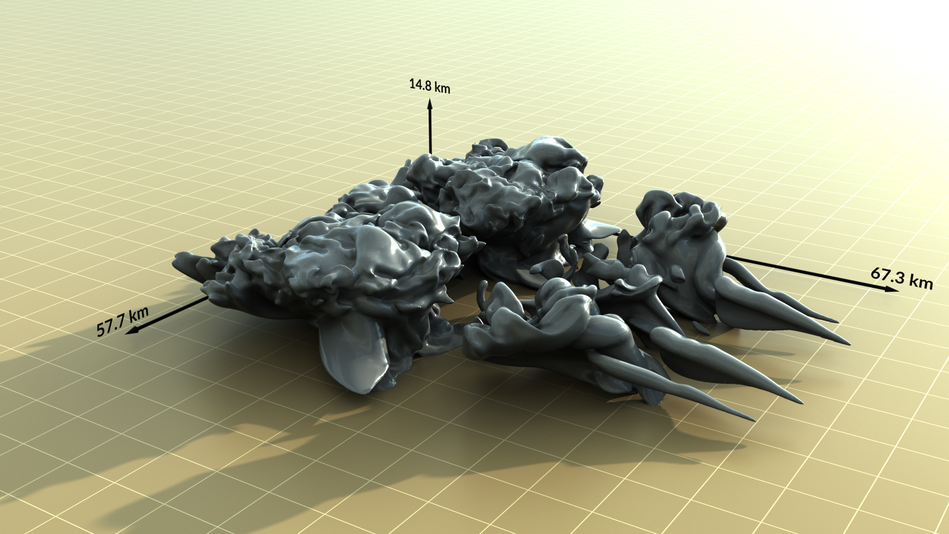
Figure 3. Still (left) and animated (right) isosurface of the sum of the thunderstorm simulation’s water vapor and liquid water fields using latitude-longitude coordinates.
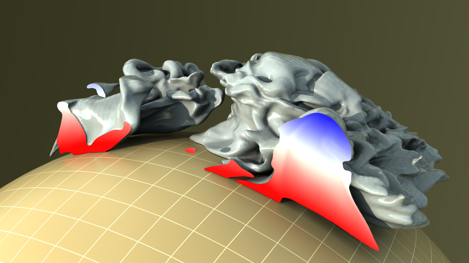
Figure 4. Still (left) and animated (right) isosurface of the sum of the thunderstorm simulation’s water vapor and liquid water fields with clipping plane and temperature gradient, using spherical coordinates.
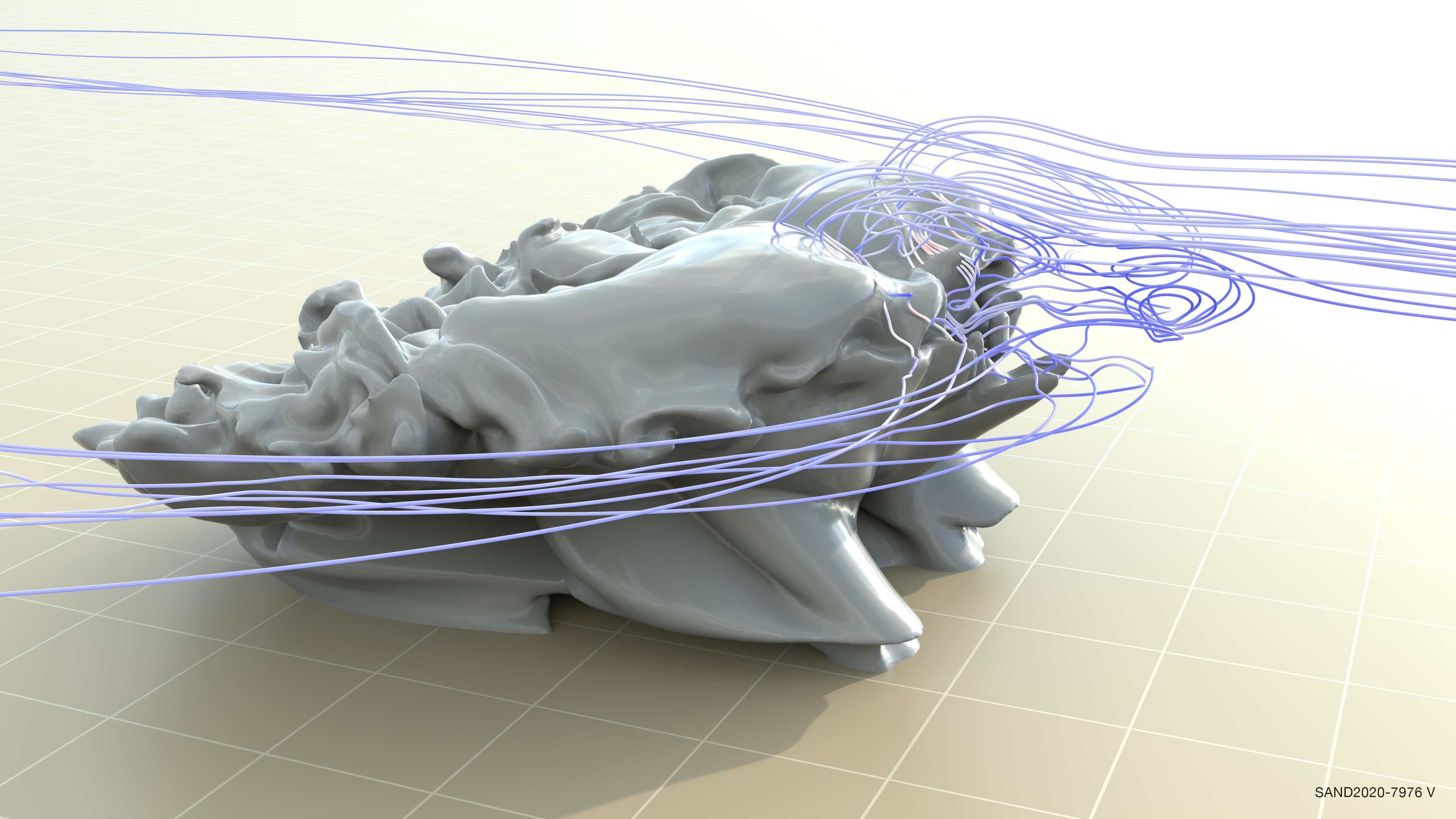
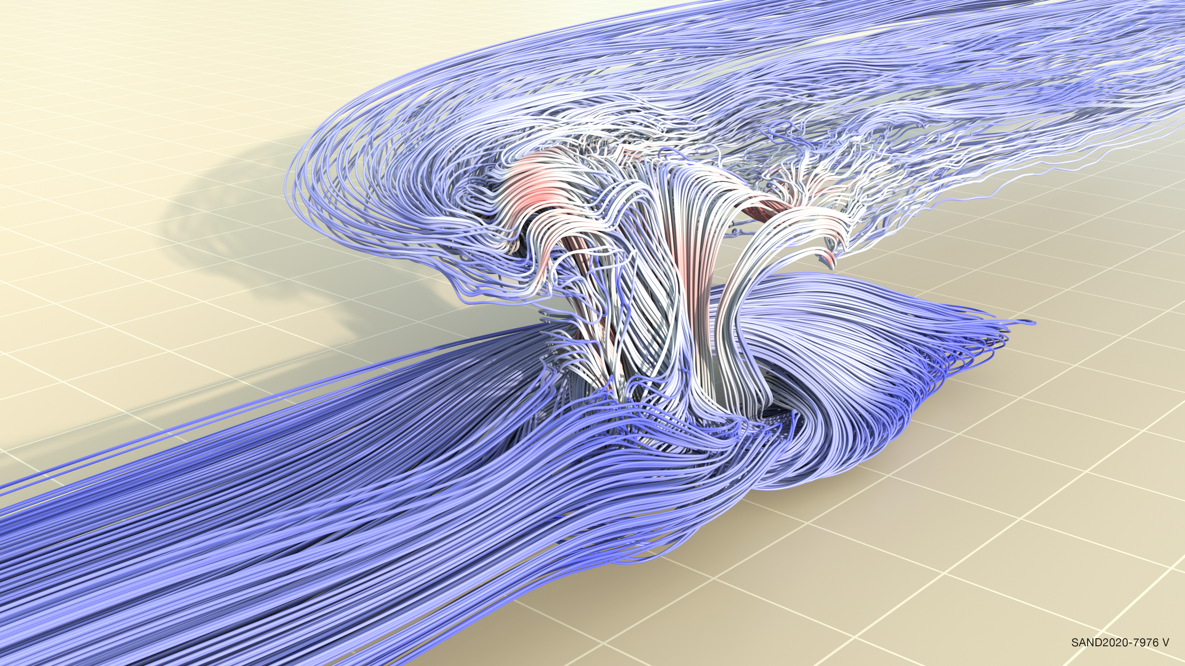
As an example of further user engagement, which can lead to scientific discovery, streamlines based on wind velocity are shown together with the condensed water mass in Figure 5 (left) to demonstrate how turbulent the near-cloud environment is. Figure 5 (right) illustrates strong updrafts that are colored red, leading to sustained storm invigoration.
Figure 5. Wind streamlines, focusing on turbulence near the leading edge of the storm (left). Wind at low altitudes is captured by the storm and rapidly rises to create the strong updrafts characteristic of supercells before being ejected from the top of the storm (right). This image focuses on one half of the storm.
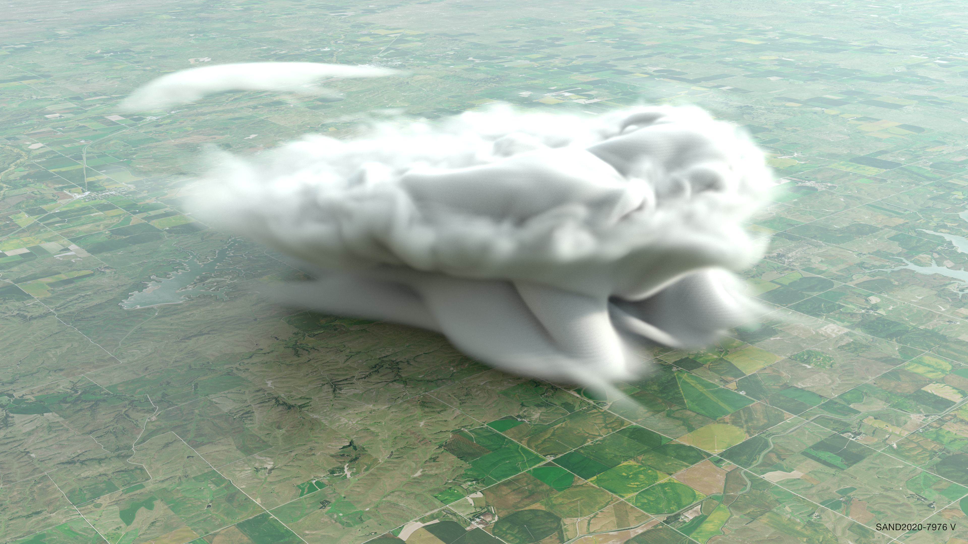
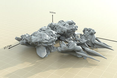
The supercell thunderstorm’s dimensions are represented schematically in Figure 3. To provide a more intuitive understanding of the size and scale of the storm, the condensed water mass was rendered over an Earth-surface scene in Figure 6.
Figure 6. Volumetric rendering of cloud water and rain water, shown with a photographic background strictly for scale. Volumetric rendering is a visual technique that shows the water concentration in the atmosphere. In this case, it is showing concentrations that are much lower than would be visible to the naked eye.
Earth’s Scale for Realism
Given the enormity of the Earth system contrasting with the local weather felt every day, an animation was sought that could link this multiscale and multidimensional perspective from the local to the global view. To do this, the freely-available Earth Studio is being used along with a free version of DaVinci Resolve to create a seamless animation that takes the viewer from a street scene out to a view of the Earth.
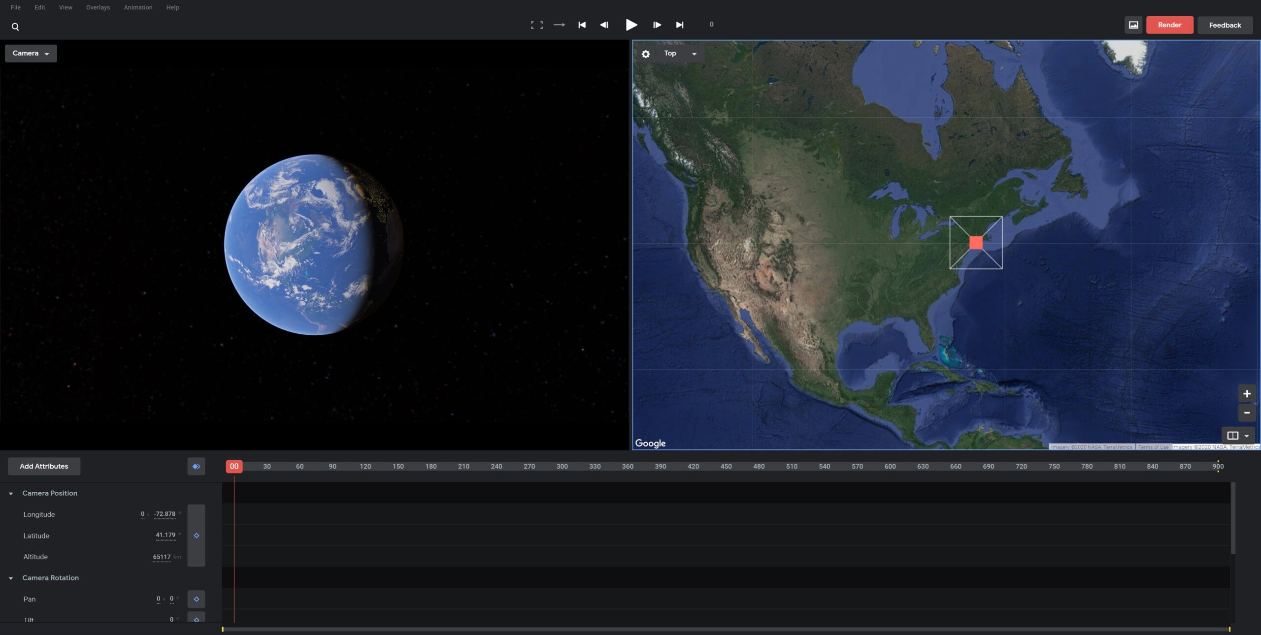
Earth Studio is a web-based application from Google (see Figure 7) and anyone with a Google account can use it. Earth Studio allows a user to very simply zoom in or out from any location on Earth. Once a location is entered, with a few additional settings, the image sequence is computed and saved to a local hard drive. These images are then imported into DaVinci Resolve, a video editor, to modify the footage and render a final video. The rendered zoom can also be inserted into an existing video project. DaVinci Resolve can also be used to add E3SM animations to an appropriate zoom in or zoom out animation.
Figure 7. Screen shot of the Earth Studio interface which allows users to record an animation of zooming in or out from any location on Earth.
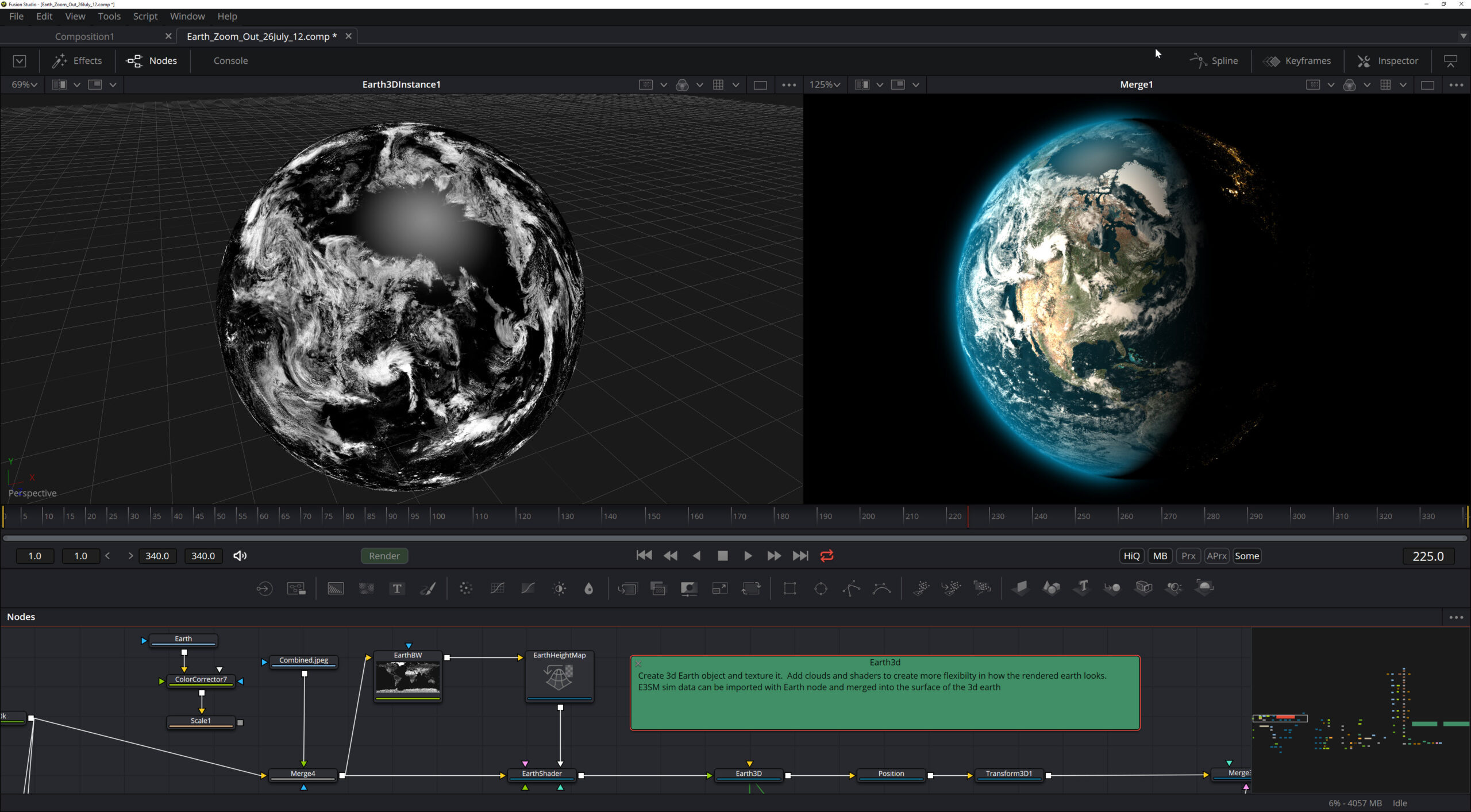
A more complex zoom-out was also developed alongside the Earth Studio zoom-out by using the Fusion compositing software. A large network of nodes combines a 3D model of Earth with NASA images of clouds used to texture the model (Figure 8). Future work would allow E3SM data to replace the NASA data and some of the Google Earth data. All layers are replicable and adjustable. Although this process is more complex than Earth Studio, this pipeline has more flexibility to create higher-quality cinematic visualizations which can convey the complexity of the Earth system to the viewer. There is work to be done on tweaking the Fusion network so that E3SM data can be imported. The potential to create impactful visualizations that incorporates E3SM data is slated for future work.
Figure 8. Fusion compositing application network of nodes. The left panel view shows a NASA image of clouds textured on to a 3D object. The right panel view shows multiple layers composited on the same 3D model, slightly rotated up to show more of North America. E3SM data can be added to the image on the right.
Summary
This project has produced animations of the coupled water cycle experiment simulation, still images and animations of thunderstorms, and a cinematic movie linking local to global all with the intention to advance scientific discovery of Earth’s Water Cycle through visualizations. New software and hardware systems were tested and utilized, seeking new ways to view multiple features of these simulations. Discoveries are underway with this new collection of images and animations which are available on e3sm.org and E3SM’s YouTube channel.
Funding
- DOE’s Office of Science, Biological and Environmental Research (BER), Earth and Environmental Systems Sciences Division (EESSD), Data Management Program, Scientific Visualization in Support of the E3SM Water Cycle Simulation Campaign Project
Computing Resources
- Theta Supercomputer at the Argonne Leadership Computing Facility (ANL)
- Cori Supercomputer at the National Energy Research Scientific Computing Center (NERSC)
- Skybridge Supercomputer (SNL)
Contact
- Erika Roesler, Sandia National Laboratories
Scientific Visualization Team
- Erika Roesler, Mark Bolstad, Brad Carvey, Timothy M. Shead, and Lauren Wheeler, Sandia National Laboratories
E3SM Climate Science Team
- Mark Taylor, Sandia National Laboratories
- Noel Keen, Lawrence Berkeley National Laboratory
- Mathew Maltrud, Los Alamos National Laboratory
- Kyle Pressel. Pacific Northwest National Laboratory


