

Modeling Ocean Mesoscale Eddies
Oceanic Scales of Motion
The ocean is host to an immense range of highly energetic motions from the global level (left panel in Figure 1), to large eddies – the “weather” of the ocean (middle two panels of Figure 1) which operates on the same general scales as thunderstorms in the atmosphere – down to very small scale turbulent mixing processes (right, Figure 1).
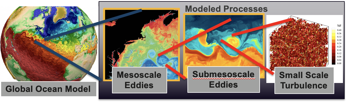
Figure 1. Schematic of scales of oceanic motion. The left panel is from an MPAS-Ocean simulation with high resolution (18 km near the equator and 6 km near the poles). Moving from left to right progressively “zooms in” to illustrate smaller scales of motion. The left three images show a bird’s eye view, while the rightmost image is a 3D view. Mesoscale eddies (6 – 100 km in diameter) are most prominent in the upper 2000 meters of the ocean where horizontal buoyancy gradients are strong and are easily seen in the MPAS-Ocean simulation as Gulf Stream rings. Submesoscale eddies (100 m – 10 km) are most prominent in the upper ocean and often form on the edge of mesoscale eddies. Small scale turbulence (<100 m) is often confined to the upper ocean, but can exist throughout the global ocean.
Mesoscale eddies range in size from five or six kilometers (in high latitudes) to approximately 100 km near the equator (Chelton et al., 1998). These eddies have a leading order impact on much of the global ocean, contributing to ocean heat transport, deep convection in the North Atlantic, and air-sea fluxes (e.g., Griffies et al., 2015, Zhu et al., 2014, Abel et al., 2017). For example, resolving mesoscale eddies in E3SMv1 drastically impacts the vertical structure of ocean heat uptake (Figure 2). When eddies are not resolved (Figure 2a), the ocean takes up heat (red) or cools (blue) at specific depths. When the resolution is increased and mesoscale eddies are resolved (Figure 2b), the location, magnitude and sign of the ocean heat content anomalies change dramatically.
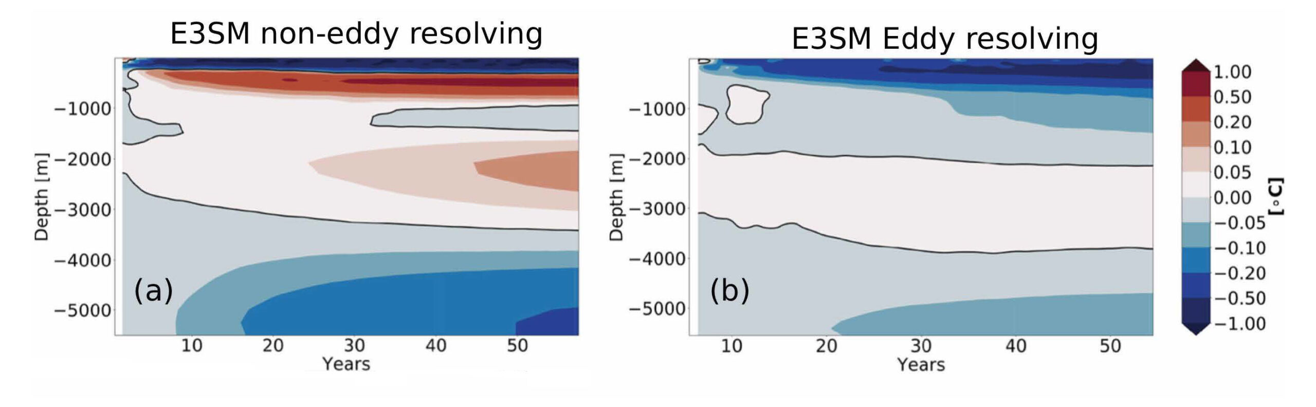
Figure 2. Globally averaged temperature anomaly (directly proportional to heat anomalies from E3SMv1). (a) Low resolution, non-eddy resolving anomalies and (b) High resolution anomalies, where mesoscale eddies are directly resolved. Red indicates ocean heat uptake and blue is heat loss. Figure adapted from (Caldwell et al., 2019).
Although it is sometimes possible to directly resolve mesoscale eddies in Earth System Model (ESM) simulations like E3SM (as illustrated in Figure 2b), global simulations at such resolution are very costly. This means that long term projections are impractical at this resolution.
Smaller scales are far from being resolved, but are equally important, especially in the upper ocean. Submesoscale eddies are 100 m – 10 km in size and are strongest near horizontal buoyancy fronts in the upper ocean. These eddies have a strong impact on vertical redistribution of heat in the ocean (Fox-Kemper et al., 2011). At the finest scales, the turbulent boundary layer (the top 100 – 1000 m of the ocean) communicates fluxes (e.g., heat, carbon dioxide) from the atmosphere or cryosphere to the deep ocean. The dynamics in this shallow top layer are crucially important for our climate, as 95% of the anthropogenically created heat in the atmosphere is communicated to the ocean through this mixing layer (Church et al., 2011).
It is critical for ESMs to include the impact of these processes in climate simulations. Despite advances in high-resolution modeling, the next 100 years are unlikely to bring researchers to the point where the underlying processes (especially submesoscale eddies and boundary layer turbulence) can be resolved in long-term climate simulations (assuming computing power continues to increase at its current rate). Therefore scientists must look to parameterizations, which are representations of unresolved processes that compute the approximate collective effect of the processes based on the resolved temperature, salinity, and currents. Unfortunately, these parameterizations are far from perfect and can lead to persistent biases in ESM simulations (Sallee et al., 2013; Large et al., 2019). The present article focuses on how to parameterize mesoscale eddies, first describing what is used by E3SM now and then discussing future directions for E3SM.
Mesoscale Eddy Parameterization
There are a number of methods used to parameterize mesoscale eddies. E3SM currently uses a combination of the Gent-McWilliams (Gent and McWilliams 1990, hereafter referred to as GM90) and Redi mixing schemes (Redi 1982). The GM90 scheme is often cast as an additional eddy advection term in the temperature and salinity equations. The parameterization acts to reduce the slope of the isopycnals thereby changing stratification, mirroring the work of eddies generated through baroclinic instability (Karsten et al., 2002). The circulation induced by mesoscale eddies is illustrated in Figure 3, where the black lines indicate a strong horizontal gradient in density and the orange lines show the stream function, which illustrates the flow. The net advective transport (shown by red arrows), tends to slump the front and increase stratification. The stream function shown in Figure 3 is the core of the GM90 parameterization.
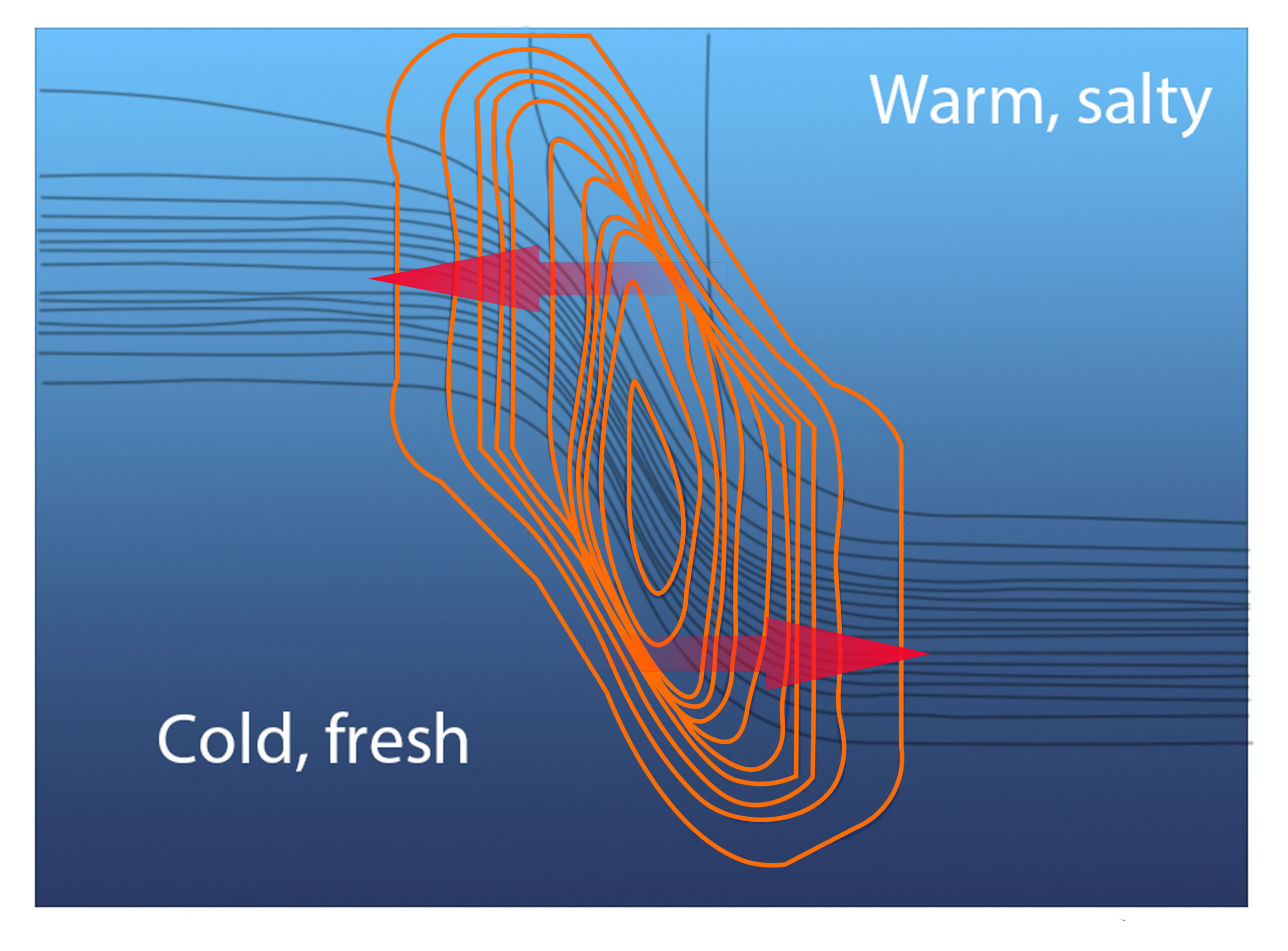
Figure 3. Schematic showing circulation induced by mesoscale eddies (image based on Gent et al., 1995). Black lines show surfaces of constant temperature, orange rings show stream function.
The Redi scheme mixes temperature and salinity along isopycnals via a rotated diffusion operator. Both GM90 and Redi are important, as they cover both advective (GM90) and diffusive (Redi) components of mixing.
Despite the long success of GM90 and Redi, questions remain on how to best implement these schemes. Within the GM90 scheme, the bolus diffusivity coefficient, which controls the strength of the advective effects, needs to be carefully constrained in order to obtain realistic model solutions (e.g., Conlon et al., in prep). Determining the best GM90 diffusivity coefficient is complex as there is evidence that the coefficient values should depend on numerous factors, for example, model resolution, latitude and longitude, vertical stratification, and background flow. Additional assumptions must be imposed for the Redi scheme, such as not allowing isopycnal slopes to exceed a critical threshold.
Recent advances have focused on whether energy considerations can help constrain and improve eddy parameterizations. For example, the GEOMETRIC (Geometry and Energetics of Ocean Mesoscale Eddies and Their Rectified Impact on Climate) scheme places an upper bound on the strength of the parameterized eddies, and is derived from the eddy energy budget. In a similar vein, Bachman (2019) suggests that a traditional GM90 eddy parameterization should be used hand-in-hand with a new momentum term, so that the effects of the parameterization on both energy and momentum are fully accounted for. Implementing these new schemes often requires solving for eddy kinetic energy via an eddy energy budget (e.g., Cessi 2008), but ensures that models represent the specific effects of unresolved eddies, while remaining consistent with basic laws of physics such as energy and momentum conservation.
Given its unstructured mesh and use of variable resolution, implementing eddy parameterizations (usually developed with regular grids in mind) in E3SM presents additional challenges. Yet, it also presents an opportunity for E3SM to push the envelope of existing parameterizations and further advance earth system modeling as a whole.
Looking Ahead
E3SM version 2 will have important improvements in how the model represents the effects of mesoscale eddies. In version 1, a rudimentary parameterization was used, with constant eddy strength across the globe. In version 2, scientists make a step toward a more physical closure where the parameterized eddy strength depends on a simplified eddy kinetic energy balance. This new parameterization will lead to a reduction in biases seen in E3SMv1 (for example, the Labrador Sea ice bias) and has already given hints of improved simulated circulation in the Southern Ocean.
New versions of E3SM will increasingly leverage variable resolution, as it is a crucial asset to better understand how global changes will impact coastal inundation or other near shore processes of national interest. As of today, the cutting-edge parameterizations in existence are unable to handle this challenge. E3SM scientists will partner with leading experts in mesoscale eddy parameterizations to improve representations of these critical eddies, allowing E3SM to address future DOE mission-critical questions.
Funding
- DOE’s Office of Science, Biological and Environmental Research (BER), Earth System Model Development (ESMD), E3SM Project
Contacts
- Luke Van Roekel, LeAnn Conlon, and Alice Barthel, Los Alamos National Laboratory