E3SM Probes Uncertainties in Ocean Surface Flux Algorithms

New research focuses on the air-sea interface. Photo by Matt Hardy on Unsplash.
Background
The atmosphere and oceans are constantly exchanging heat, water, momentum and gases like carbon dioxide. Atmospheric turbulence – the chaotic whirling of air superimposed on the mean wind – is central to the physics of these exchanges. However, because this turbulence occurs on scales from millimeters to kilometers, it is not possible for numerical weather, climate and Earth system models to directly simulate the turbulent exchanges. Instead, models calculate turbulent fluxes with “bulk parameterizations”, which estimate fluxes based on the large-scale average properties (as opposed to the small-scale turbulent fluctuations) like air temperature and humidity, wind speed and sea surface temperature.
Many bulk parameterizations have been developed over recent decades and they share a common theoretical underpinning – called Monin-Obukhov similarity theory. However, the parameterizations have many differences in their implementation of the underlying theory. While the differences between parameterizations are well understood in idealized comparisons, model sensitivity to the choice of parameterization is less well understood and can be complicated. This is because small flux differences may result in changes to atmosphere model processes (e.g., cloud formation and precipitation) and ocean model processes (e.g., deep water formation in high latitudes) which can, in turn, affect the fluxes and form a feedback loop. A few studies have looked at model sensitivity in individual processes (e.g., deep water formation in the high latitude oceans) or individual aspects of parameterization design (e.g., roughness length), but more general model studies of widely used bulk parameterizations had until recently been lacking.
E3SM Experiments
In a recent study published in Frontiers in Marine Science, researchers compared E3SM simulations with three different bulk parameterizations, looking at the sensitivity of both ocean and atmosphere models. The control experiments used the bulk parameterization from E3SM v1. The two new parameterization algorithms were COARE (from the Coupled Ocean-Atmosphere Response Experiment field campaign) and UA (developed at the University of Arizona). The code for these parameterizations was added to E3SM specifically for studies of this kind. For each parameterization, one atmosphere simulation and one ocean simulation were performed.
Atmosphere simulations were forced with prescribed ocean and sea ice fields (e.g., sea surface temperature), while ocean simulations were forced with prescribed atmosphere and river runoff fields. This allows the feedbacks between fluxes and the atmosphere model to be isolated from feedbacks between fluxes and the ocean model.
Flux Changes
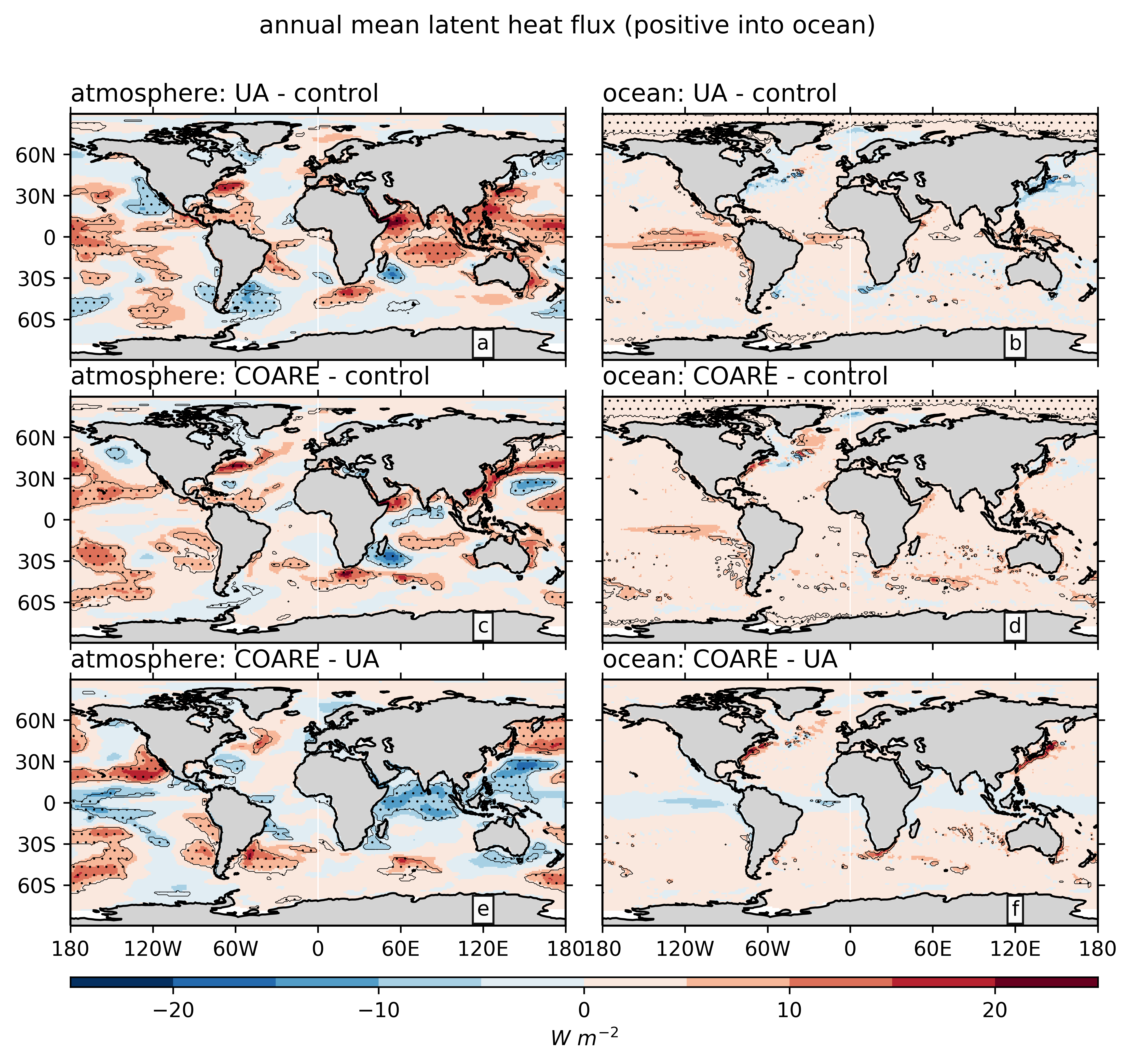
Regions with large flux differences (Figure 1) show where the parameterizations vary significantly. Some regions have large differences across all atmosphere and ocean simulations, while other regions only show up in a subset of the comparisons. For example, western boundary currents like the Gulf Stream and Kuroshio current have quite large differences across both ocean and atmosphere simulations and across all pairs of parameterizations. The tropical Indo-Pacific region is highlighted by the atmosphere simulations, while the tropical eastern Pacific is more prominent in the ocean simulation differences. What unites many of these regions, however, is that they are recognized as somewhat unusual cases in the flux parameterization literature and are the subject of ongoing observational study.

Figure 1. Differences in annual mean latent heat flux climatology between simulations with different bulk flux algorithms. The atmosphere and ocean simulation results are shown in left and right panels, respectively. Stippling designates regions where the absolute value of the difference is larger than the interannual standard deviation from the E3SMv1 pre-industrial control run. Latent heat flux is a measure of the energy exchange involved in the evaporation process. Changes are larger between pairs of atmosphere simulations (left column) than pairs of ocean simulations (right).
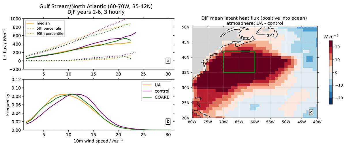
In general, the flux differences among the three atmosphere simulations were larger than among the three ocean simulations. This is because the wind speed, which is a strong determinant of the strength of turbulence, can vary freely in the atmosphere simulations (Figure 2) while it is pre-determined by “forcing” data in the ocean simulations. Interestingly, this opens up the possibility that the ocean sensitivity may be larger in coupled simulations than in the forced ocean simulations performed here.

Figure 2. (a) Latent heat flux quantiles, as functions of 10-m wind speed, and (b) 10-m wind speed distributions, for the three atmosphere simulations in a region around the Gulf Stream (60−70°W, 35−42°N). (c) December to February multi-year mean latent heat flux difference between UA and control atmosphere simulations, with the region used in (a, b) shown by the green box. Note the differing sign conventions: evaporation corresponds to positive values in (a) but negative values in (c). The changes in (c) occur due to a combination of changes in the latent heat flux at any particular wind speed (solid yellow line lower than solid purple line in a) and changes in the frequency of each wind speed (solid yellow line shifted left of solid purple line in b).
Atmosphere and Ocean Changes
The flux changes caused by the different parameterizations led to a host of other changes in the atmosphere and ocean model behavior, including some well away from the surface where the flux changes act. In the atmosphere simulations, significant changes occurred in the global energy and water cycles. For example, evaporation and precipitation differed, both in the global mean and regional patterns. At the same time, the global distribution of clouds was affected, changing the balance of radiation at the top of the atmosphere. In the ocean, heat uptake and patterns of heat transport by ocean currents were both affected.
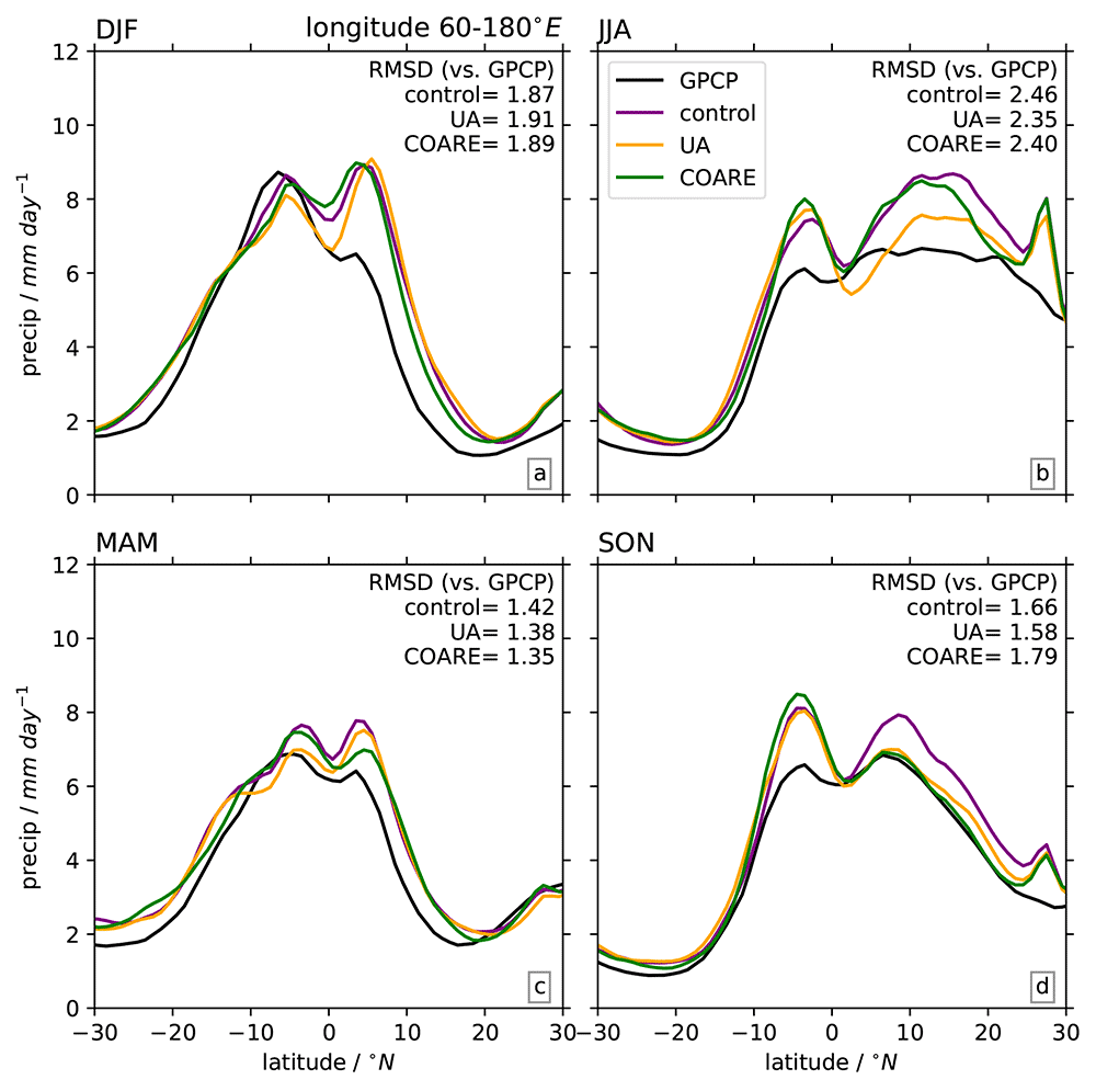
Compared to the control experiment, COARE and UA improved upon several model biases: COARE significantly reduced the global mean evaporation which in turn reduced the global mean precipitation – taking the model value closer to the observed value (albeit, still larger than the observed value). UA meanwhile resulted in the biggest improvement to top-of-atmosphere radiation balance, and a slight reduction in the model biases of ocean heat transport. However, no single parameterization was best across all metrics, all seasons or all regions (Figure 3), which reflects the inherent uncertainties in the bulk parameterization method and also the far-reaching consequences of these uncertainties in Earth system models.

Figure 3. Zonal mean, seasonal mean precipitation from the three atmosphere simulations and GPCP observational data: (a) December to February; (b) June to August; (c) March to May; (d) September to November. The zonal sector considered is 60°E to 180°E. GPCP data were bilinearly interpolated to the same 1° grid as the other data before calculating. Text in each panel shows the area-weighted root mean square difference (RMSD), in millimeters (mm) per day, between each model and the GPCP data. These statistics demonstrate that no single algorithm performs best in all seasons.
Impact and Future Work
This study sheds light on the type and magnitude of model uncertainties that arise due to limitations in how accurately scientists can calculate ocean surface fluxes. For example, the rate of ocean heat uptake and regional precipitation patterns differ between simulations with different bulk parameterizations. This work begins to provide insight into how projections of global warming and changes in precipitation extremes may be affected by the choice of bulk parameterization. Understanding these implications more will take coupled model simulations (rather than the separate “forced” model simulations used here), with longer duration. Such coupled simulations may be the subject of future studies with E3SM and other Earth system models.
The other impact of this study is the potential insight it offers for bulk parameterization design. A few regions and physical regimes (e.g., western boundary currents; Figures 1 and 2) consistently stick out as having large differences between the parameterizations, so these regions are ripe for further observational study and continued refinement of parameterization design.
Publication
- Reeves Eyre J. E. J., Zeng, X., & Zhang, K. (2021). Ocean Surface Flux Algorithm Effects on Earth System Model Energy and Water Cycles. Frontiers in Marine Science. 8:642804. https://doi.org/10.3389/fmars.2021.642804
Funding
- DOE’s Office of Science, Biological and Environmental Research (BER), Earth System Model Development (ESMD), E3SM Project
Contacts
- Jack Reeves Eyre, Cooperative Institute for Climate, Ocean and Ecosystem Studies, University of Washington.


