

The DOE E3SM Version 2.1: Overview and Assessment of the Impacts of Parameterized Ocean Submesoscales
In March 2025, a manuscript that documents and evaluates the E3SM Version 2.1 release in its lower resolution configurations (v2.1 LR) was published in Geoscientific Model Development (doi: 10.5194/gmd-18-1613-2025). This publication serves as the main reference for the E3SMv2.1 model, with additional papers documenting the biogeochemistry and cryosphere configurations to follow in the near future.
Key Takeaways
- Version 2.1 of the U.S. Department of Energy’s Energy Exascale Earth System Model (E3SM) adds the Fox-Kemper et al. (2011) mixed-layer eddy parameterization, which restratifies the ocean surface layer through an overturning streamfunction.
- Results include ocean surface layer bias reduction in temperature, salinity, and sea ice extent in the North Atlantic; a small strengthening of the Atlantic meridional overturning circulation; and improvements to many atmospheric climatological variables.
Background
The U.S. Department of Energy (DOE) Energy Exascale Earth System Model (E3SM) project aims to meet the energy mission and science needs of the DOE using state-of-the-art DOE computing resources. Version 1 (E3SMv1) was released in 2018, and while the land model and coupler were similar to those in CESM (Community Earth System Model; Hurrell et al., 2013; Danabasoglu et al., 2020), the river routing, ocean, sea ice, atmospheric physics, atmospheric dynamical core, and stratospheric chemistry were significantly different. Both lower-resolution (110 km atmosphere and 60–30 km ocean) and higher-resolution (25 km atmosphere and 18–6 km ocean) configurations were released (Golaz et al., 2019; Caldwell et al., 2019), as were biogeochemical and cryosphere configurations (Burrows et al., 2020; Comeau et al., 2022). Following version 1, version 2 (E3SMv2) was released in 2022 with significant improvements to the modeled earth system state, including a 2× speedup from E3SMv1 (Golaz et al., 2022). For this version, a lower-resolution configuration and a North American regionally refined configuration (Tang et al., 2023) have been released, with plans for a biogeochemistry configuration with interactive carbon and nutrient cycles and a cryosphere configuration with regional refinement over the Southern Ocean in the future.
Version 2.1 (E3SMv2.1) builds on E3SMv2 (Golaz et al., 2022) with several changes, most notably the addition of the so-called “Fox-Kemper2011” mixed-layer eddy (MLE) parameterization (hereafter referred to as FK11; Fox-Kemper et al., 2008, 2011). Shallow, ageostrophic baroclinic instabilities, often referred to as submesoscale instabilities, develop on lateral density fronts in the weakly stratified surface mixed layer. Once they become finite in amplitude, the resulting mixed-layer eddies slump the fronts, releasing potential energy and contributing to the restratification and shoaling of the mixed layer (Boccaletti et al., 2007). Due to their small spatial scales (𝒪(10 km)), these submesoscale instabilities and their effects are not explicitly resolved in global ocean models, even at “eddy-resolving” resolutions, and thus they need to be parameterized. Fox-Kemper et al. (2008) proposed a parameterization in the form of an overturning streamfunction to mimic the MLE fluxes of density and other tracers. By construction, this overturning streamfunction acts to slump isopycnals (layers of constant potential density) and enhance restratification of the mixed layer.
This publication largely focuses on documenting the implementation of the MLE parameterization from FK11 in the ocean component of the E3SM, the Model for Prediction Across Scales – Ocean (MPAS-Ocean). The researchers investigated the response of the coupled model to the MLE fluxes, with a particular focus on high-latitude convection and large-scale ocean circulation, including the Atlantic Meridional Overturning Circulation (AMOC).
Overall, the v2.1 configuration resulted in some improvements to North Atlantic Ocean biases, particularly sea surface temperature (SST) and sea surface salinity (SSS) (Figs. 1 and 2), which resulted in improved sea-ice concentration in the North Atlantic (Fig. 3).
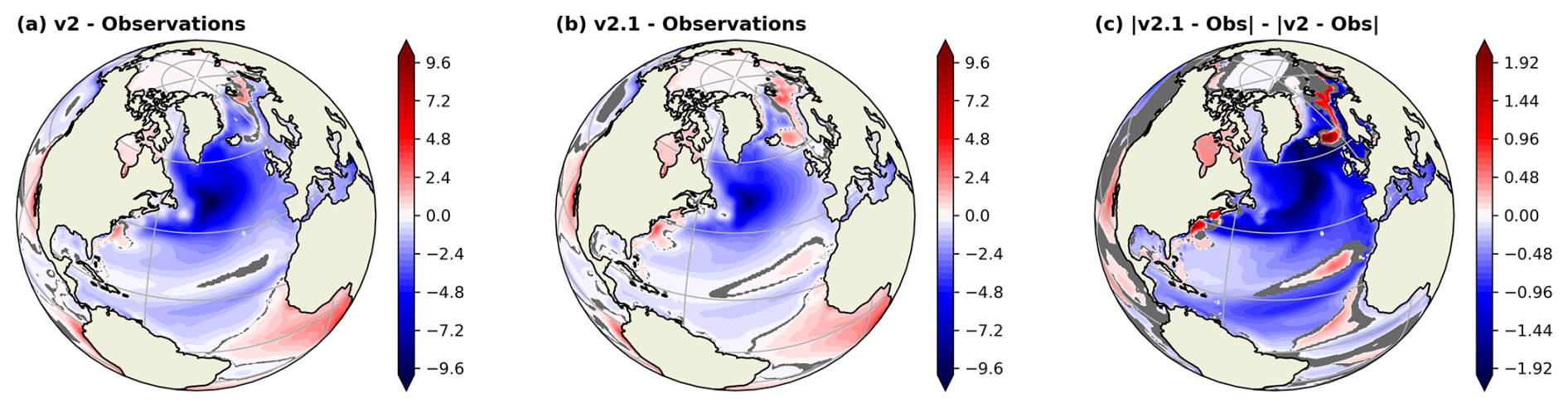
Figure 1. Annual climatological SST biases (°C) with respect to observations for the (a) v2 and (b) v2.1 configurations. (c) The change in SST biases between the v2.1 and v2 configurations. Light gray denote no data, dark gray – no significant difference.
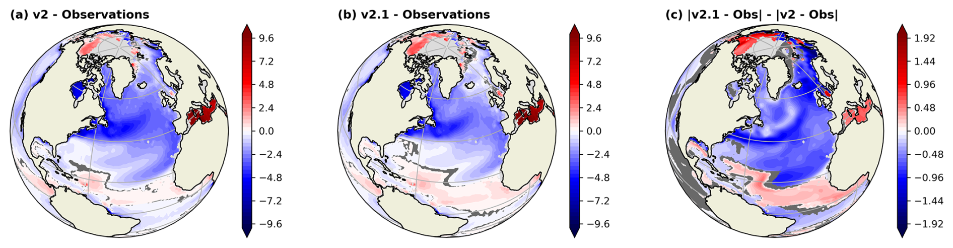
Figure 2. The same as Fig. 1 but for SSS (psu).
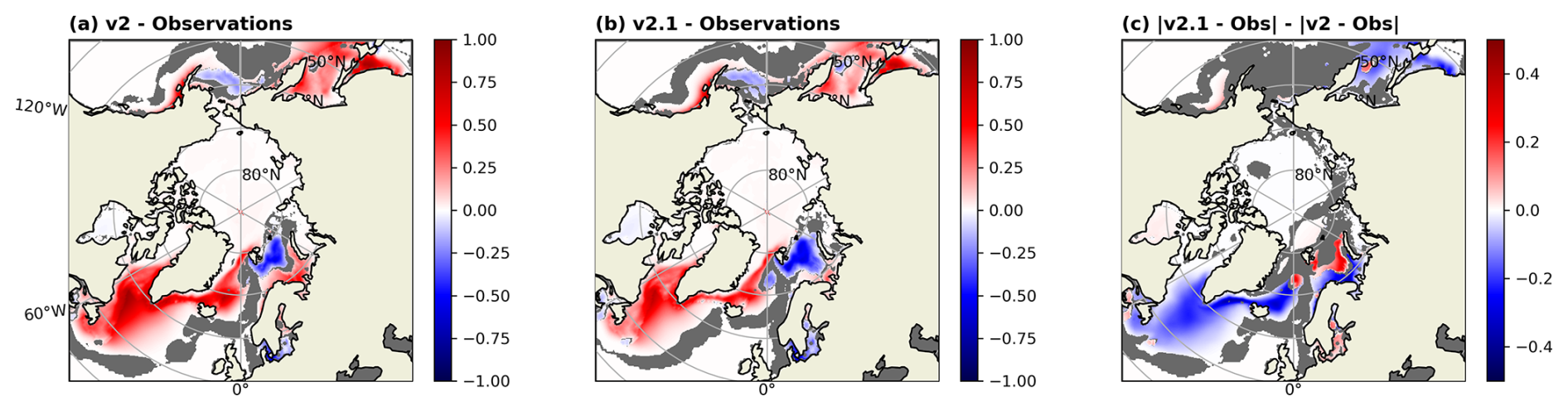
Figure 3. The same as Fig. 1 but for sea-ice concentration (fraction).
Changes in mixed layer depth (MLD) biases were as expected, mirroring FK11 with a general shoaling of the mixed layer (Fox-Kemper et al., 2011) visible in many regions (Fig. 4), although coupled feedbacks led to regional deepening of the MLD that reduced the mean MLD bias globally (Fig. 5). Additionally, although MLD is underestimated in comparison to observations in most regions, it does not appear to lead to any widespread degradation in the mean state.
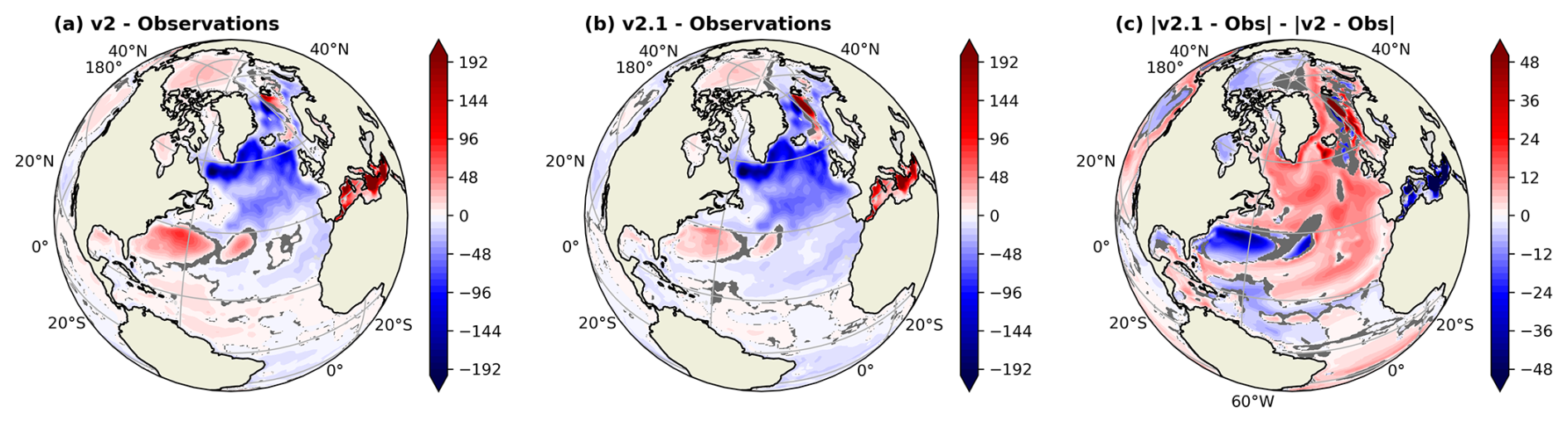
Figure 4. The same as Fig. 1 but for MLD (m).

Figure 5. Correlations (top row) and RMSE (root mean square error; bottom row) of the global MLD (m), SST (°C), SSS (psu), sea surface hight (SSH; cm), and eddy kinetic energy (EKE; kg2 s−2) for the v2 (blue markers) and v2.1 (orange markers) historical ensemble simulations relative to observations. Symbols indicate individual ensemble members and thick, open-circle indicate the multi-realization averages of the five historical ensemble members over the 1980–2014.
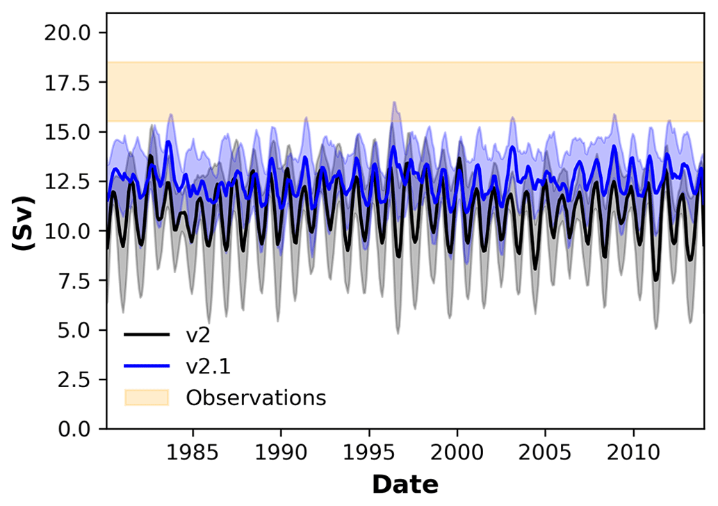
Figure 6. Time series of the maximum AMOC (Sv) at 26.5° N for the E3SM v2 configuration (black), the E3SM v2.1 configuration (blue), and an estimate of the observational range (orange) over the 1980–2014 period. Thick lines denote the ensemble mean, while shading illustrates 1 standard deviation from that mean after a 12-month smoothing is applied.
AMOC magnitude increased slightly with the addition of the MLE parameterization (Fig. 6). This is expected since the direct effect of the FK11 parameterization on AMOC appears to be model dependent and tends to either stabilize or minimally affect AMOC (Fox-Kemper et al., 2011). This effect holds for the v2.1 ensemble of simulations, which showed less variability in AMOC overall. Differences in AMOC may at least in part be due to a relocation of the site of deep convection from the Labrador and Irminger seas and North Atlantic to the Nordic Seas (Fox-Kemper et al., 2011). This hypothesis aligns with changes we saw in our modeled MLDs in v2.1 when compared with v2.
There appear to be differences in MLD in the Nordic Seas that are separate from the overall MLD shoaling created in v2.1, indicating potential changes in deep-water formation there (Fig. 7). Similar to Fox-Kemper et al. (2011), we also saw deep convection occurring in the Nordic Seas rather than in the Labrador and Irminger seas.
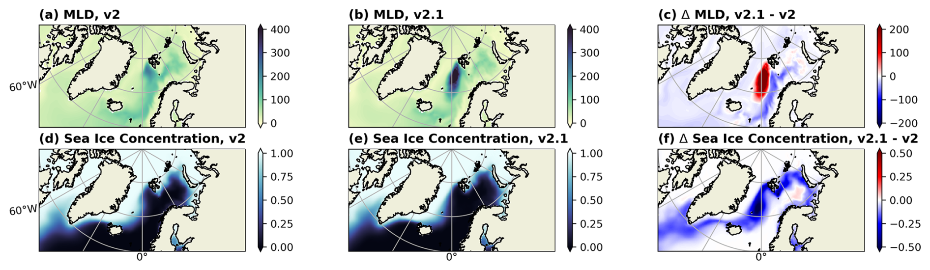
Figure 7. Annual climatological (a–b) MLD (m) and (d–e) sea-ice concentration (fraction) in the Nordic Seas for the (a, d) v2 and (b, e) v2.1 configurations. Change in (c) MLD and (f) sea-ice concentration between the v2.1 and v2 configurations.
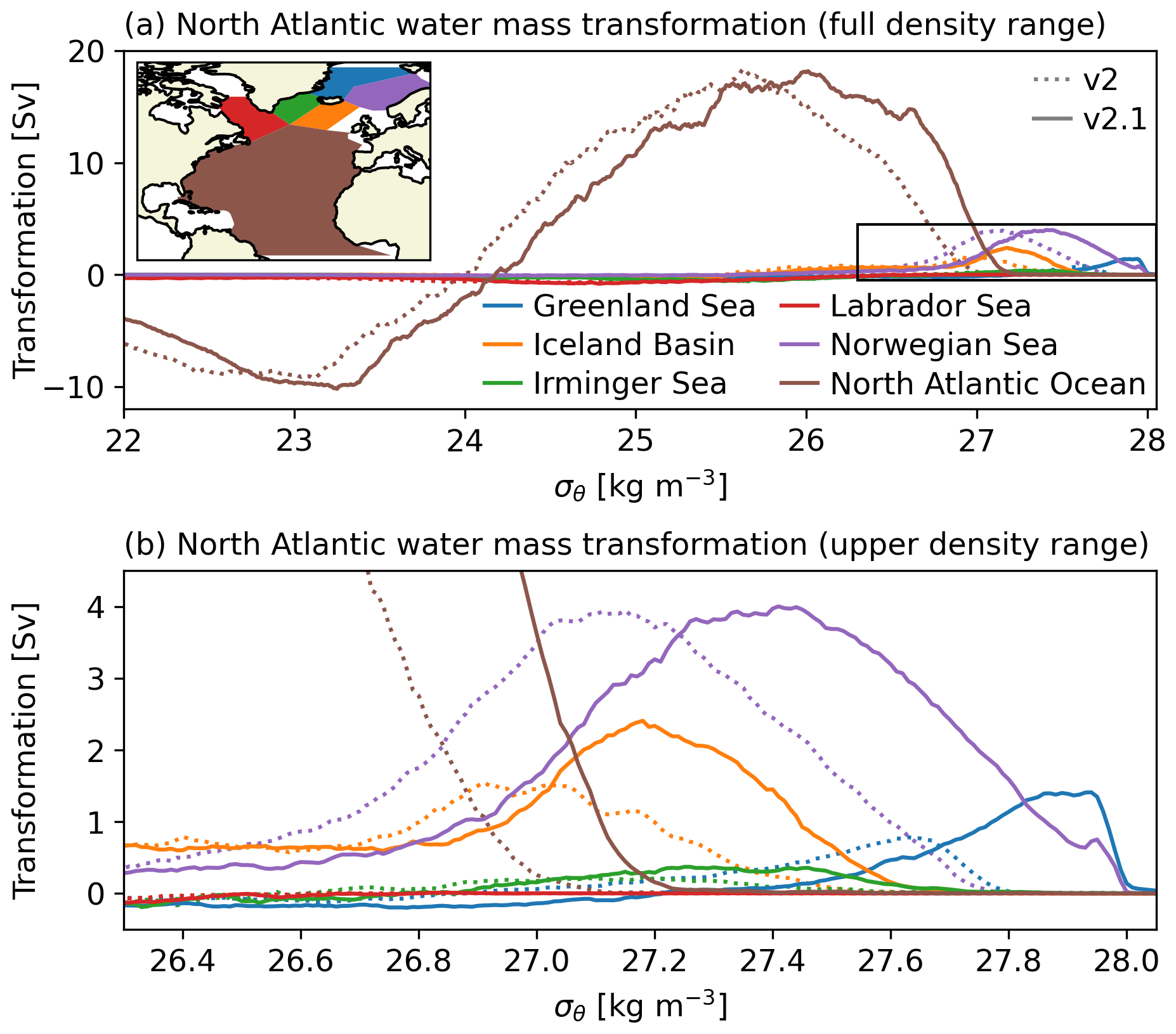
Figure 8. Surface water mass transformation in select North Atlantic basins in the v2.1 (solid lines) and v2 (dotted lines) configurations averaged over the 33-year piControl Ext runs (years 501–533). Panel (a) shows the full analyzed density range, while panel (b) zooms in on the higher density classes relevant to the subpolar basins shown. The extent of each region is shown in the map inset in panel (a). The x axis σθ is the surface-referenced potential density minus 1000 kg m−3.
The water mass transformation analysis shows changes in deep-water formation, particularly in the North Atlantic and Norwegian Sea, with more dense water being formed in v2.1 than in v2 (Fig. 8). While it is not clear why this is the case, it does explain why our modeled AMOC improves slightly while not drastically altering the North Atlantic Subpolar Gyre. If increased deep-water formation was occurring in the Labrador and Irminger seas, we would expect to see a greater decrease in the SSS, SST, and sea-ice biases there.
The passive tracer transport analysis in Fig. 9 for v2.1 indicates that the increased deep convection may not translate to a better AMOC because the dense water formed is transported northward into the Arctic rather than towards the south. Comparison of tracer advection from v2 to v2.1 shows deep northward convection from the Barents Sea into the Arctic in v2.1 (this does not occur in v2). Future work will attempt to elucidate the mechanisms behind this shift in deep-water formation.
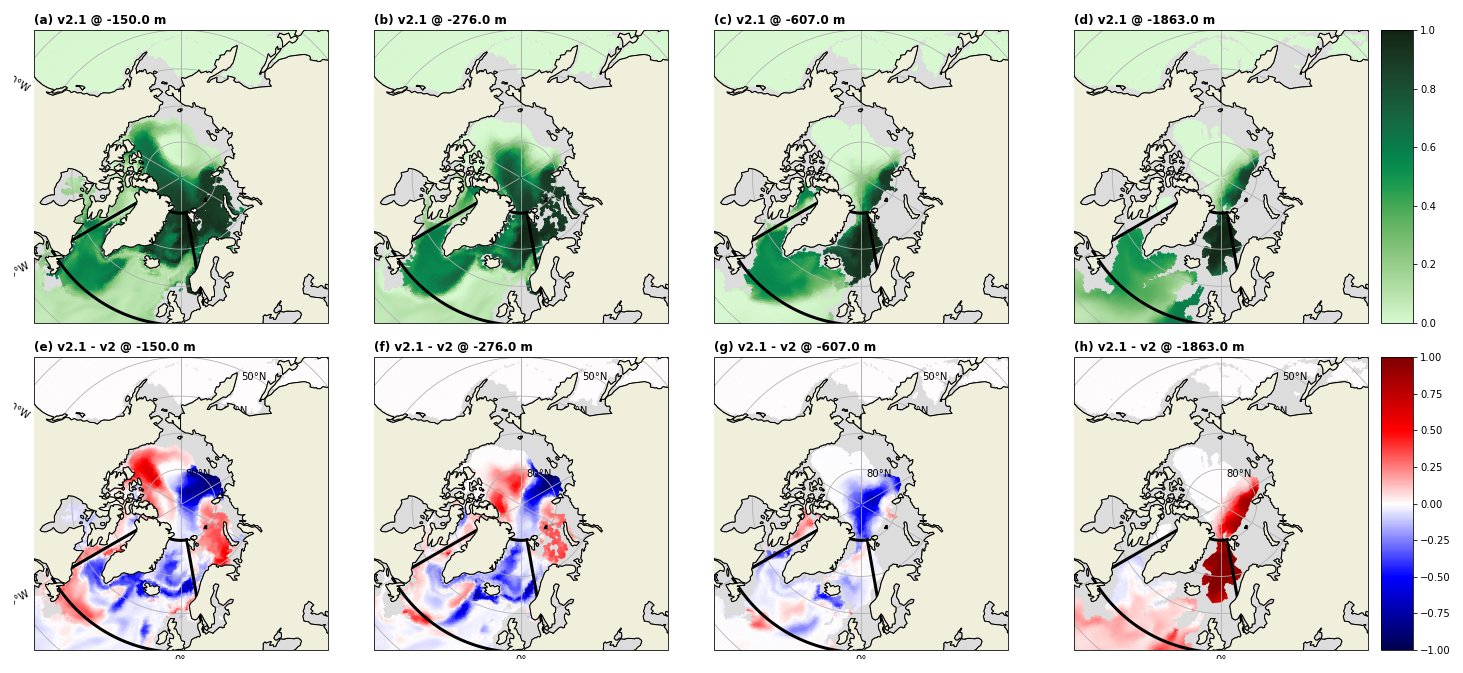
Figure 9. (a–d) Tracer concentration in the v2.1 configuration and (e–h) the change in concentration between the v2.1 and v2 configurations 33 years after tracer initiation at depths of (a, e) −150 m, (b, f) −276 m,(c, g) −607 m, and (d, h) −1863 m. Thick black boxes indicate the extent of the tracer surface forcing, while light gray shading denotes bottom topography at that model depth.
The team applied the Program for Coordinated Model Diagnosis and Intercomparison (PCMDI) Metrics Package (PMP; Lee et al., 2024), which is an open-source Python software package that provides quick-look objective comparisons of Earth system models with one another and with observations. The results indicate that the climatological characteristics of many surface and atmospheric fields in E3SMv2.1 (precipitation, sea level pressure, radiation at the surface and the top of the atmosphere, air temperature at 200 and 850 hPa, surface air temperature, surface temperature, wind components at 200 and 850 hPa, and 500 hPa geopotential height) have improved compared to v2 (Fig. 10). Using PMP, the team also examined the model performance of seven interannual extratropical modes of variability, including the atmospheric-based Northern Annular Mode (NAM), North Atlantic Oscillation (NAO), Pacific–North America pattern (PNA), North Pacific Oscillation (NPO), and Southern Annular Mode (SAM) and two modes based on SST, i.e., the Pacific Decadal Oscillation (PDO) and the North Pacific Gyre Oscillation (NPGO). The results suggest noticeable improvement in the NAO and NAM; however, for most modes and seasons we find the large-scale extratropical modes of variability in E3SMv2.1 are not significantly different from v2 (Fig. 11).
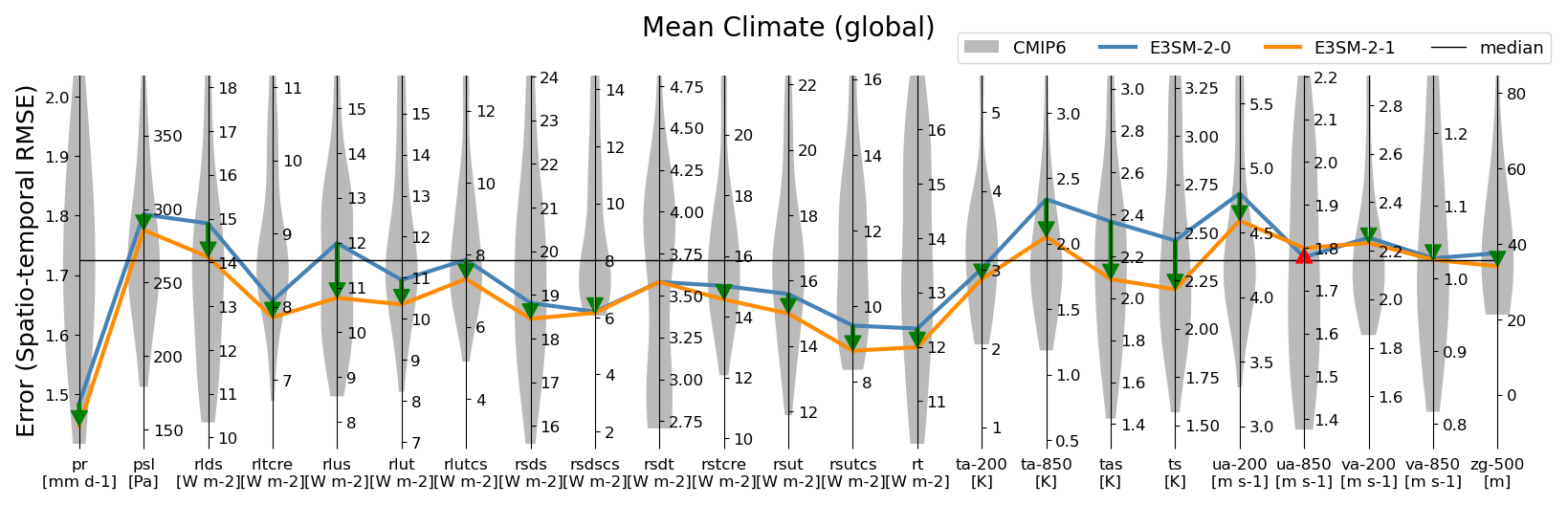
Figure 10. The PMP Parallel Coordinate Plot for global mean state evaluation, showing the spatiotemporal RMSE. Each vertical axis represents a different variable (for details see to Table 1). RMSEs are constructed using the five v2 (blue) and v2.1 (orange) historical ensemble members over 1981–2005. Improvement (degradation) in v2.1 compared to v2 is shown as a downward green (upward red) arrow between lines. The midpoint of each vertical axis is shifted to represent the median result from the CMIP6 multi-model ensemble (horizontal black line), with the axis range stretched to the minimum and maximum from the median CMIP6 for visual consistency. The inter-model distributions of CMIP6 model performance are shown as shaded violin plots along each vertical axis.
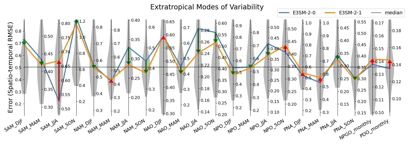
Figure 11. The PMP Parallel Coordinate Plot for extratropical modes of variability evaluation, showing the spatiotemporal RMSE. Each vertical axis represents a different mode and season. Analysis is constructed using the five v2 historical and v2.1 historical ensemble members over the 1900–2005 time period. Colors, arrows, shading and other details are the same as in Fig 10.
Data Availability
The E3SM code is available at E3SM GitHub, and the model versions used for the simulations presented here are E3SM v2.1 and E3SM v2. A full list of all code changes made from v2 to v2.1 can be found on GitHub. Information about running the model is available at running-e3sm-guide. The simulation data used for this paper are published as part of CMIP6 through the Earth System Grid Federation (ESGF). The data are available from ESGF search. Preliminary analysis of the ocean component MPAS-Ocean was performed using MPAS-Analysis.
Reference
Smith, K. M., Barthel, A. M., Conlon, L. M., Van Roekel, L. P., et al. (2025). The DOE E3SM version 2.1: overview and assessment of the impacts of parameterized ocean submesoscales. Geosci. Model Dev., 18, 1613–1633, https://doi.org/10.5194/gmd-18-1613-2025.
Related Articles
This article is a part of the E3SM “Floating Points” Newsletter, to read the full Newsletter check: