

Overview Paper on Cryosphere Configuration
In January 2022, a paper that documents and evaluates the performance of the E3SM Version 1.2 Cryosphere configuration was published in the Journal of Advances in Modeling Earth Systems (JAMES), DOI: 10.1029/2021MS002468.
This paper will serve as the main reference for the E3SMv1.2-Cryosphere model, in particular for the new capability of simulating ice-shelf basal melting under Antarctic ice shelves.
Background
The future of the Antarctic Ice Sheet (AIS) has the potential to have broad impacts on global earth system, perhaps most notably in contributing to sea-level change. The current generation of Earth System Models (ESMs) does not accurately represent the two primary means in which ice is lost from the AIS — through melting at the base of ice shelves floating on the ocean and the calving of icebergs. Lack of explicit representation of the processes by which freshwater (and the associated heat) are exchanged between the AIS and the rest of the system in an ESM limits the ability to make projections that incorporate the impacts of the AIS in a changing earth system.
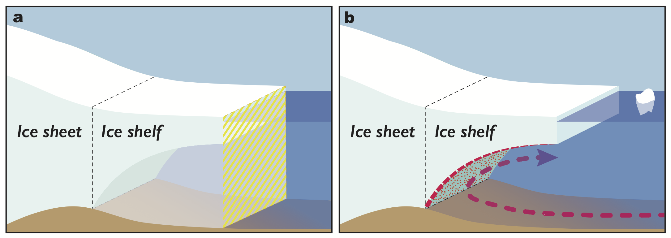
Figure 1: Schematic, profile view of a marine ice-sheet margin illustrating the representation of ice shelves in E3SM. In both panels, the black dashed lines represent a vertical plane passing through the grounding line, the location at which the ice sheet goes afloat via buoyancy.
a) Prior to the improvements discussed in this paper, the ocean domain in E3SM, as in most ESMs, ended with a vertical wall at the ice-shelf calving front (yellow-striped plane in (a)).
b) The new configuration of E3SM includes circulation of the ocean within static ice-shelf cavities and prognostic ice-shelf basal melt fluxes into the ocean. The new configuration also includes realistic, prescribed iceberg melt fluxes.
E3SMv1.2 – Cryosphere Configuration
Relative to the standard E3SMv1 configuration, the v1.2 Cryosphere configuration has been developed to improve the representation of ice-ocean interactions with the AIS. The scientists added the capability to simulate Antarctic ice-shelf basal melting, which has been implemented through simulating the ocean circulation within static Antarctic ice-shelf cavities (Fig. 1), allowing for the calculation of ice-shelf basal melt rates from the associated heat and freshwater fluxes. In addition, the ability to prescribe the Southern Ocean freshwater flux resulting from iceberg melt was added, allowing for a realistic representation of the other dominant mass loss process from the AIS. These two capabilities replace the standard representation of AIS runoff in E3SMv1, which routes rain and snow that falls on Antarctica to the nearest coastal grid cell.
Summary of Results
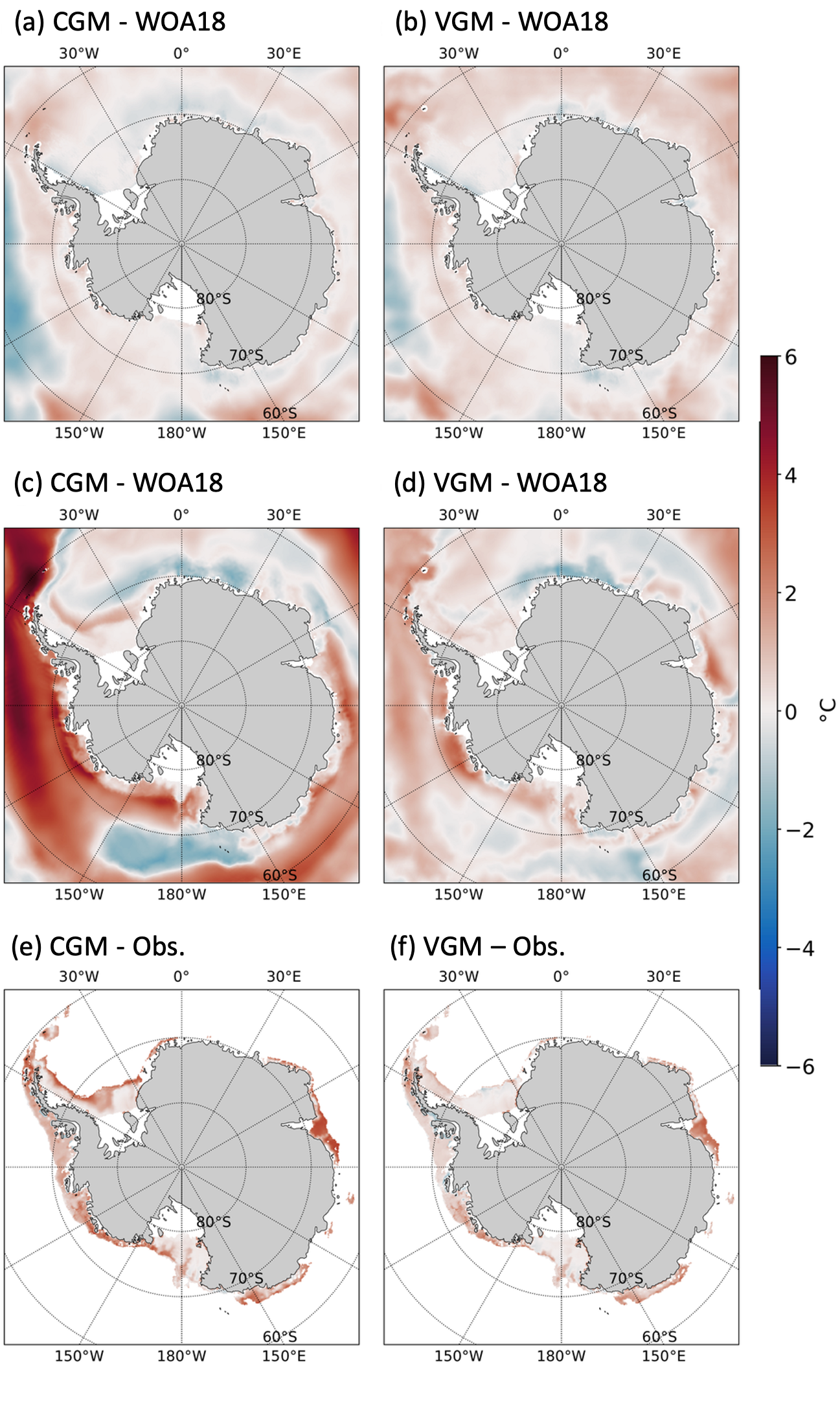
Figure 2: Differences between simulated SST (a,b) and potential temperature at 200m (c,d) from the CGM (left column) and VGM (right column) simulations, respectively, and WOA18 (Boyer et al 2018) annual climatology; differences between simulated potential temperature at the seafloor from the CGM (e), VGM (f) simulations and the Schmidtko et al 2014 observational data set (observations available on the continental shelf only).
In the paper, the researchers present the result of a pair of fully coupled, 200 year simulations under pre-industrial forcing at standard resolution, which includes atmosphere and land (110 km grid spacing), ocean and sea ice (60 km in the mid-latitudes and 30 km at the equator and poles), and river transport (55 km) models. At this resolution for the ocean, mesoscale eddies are not resolved, and are represented by the Gent-McWilliams (GM) parameterization. The first simulation uses a Constant Gent-McWilliams (CGM) bolus kappa coefficient, which is standard in E3SMv1. The second uses a Variable GM parameterization (VGM), where the kappa coefficient is stratification dependent.
First, a baseline model validation of the regional system around Antarctica was established. Ice-shelf basal melt rates, the primary metrics of interest, are driven by surrounding ocean properties, particularly on the continental shelf. In the CGM simulation, there is a general warm subsurface ocean bias in the Southern Ocean around Antarctica (Figure 2c,e). In the VGM simulation, a better representation of the spatial variability of eddy-induced transport reduces biases in water mass properties on the Antarctic continental shelf (Figure 2d,f). While the SST bias is similar in CGM and VGM (Figure 2a,b), CGM has a fresh bias in surface salinity that is substantially reduced in VGM (not shown here).
In terms of simulated ice-shelf basal melt rates, high sensitivity of modeled ocean/ice shelf interactions to the ocean state and the associated temperature and salinity biases were found. In particular, these biases can result in a rapid transition to a high basal melt regime under the Filchner-Ronne Ice Shelf (FRIS) in the CGM simulation (Figure 3d; blue line), presenting a significant challenge to a realistic representation of the ocean/ice shelf system in a coupled ESM. With the reduction of ocean biases in the VGM simulation, this rapid transition in melt regime under FRIS does not occur, and simulated basal melt rates remain within present-day observations (Figure 3d; orange line).
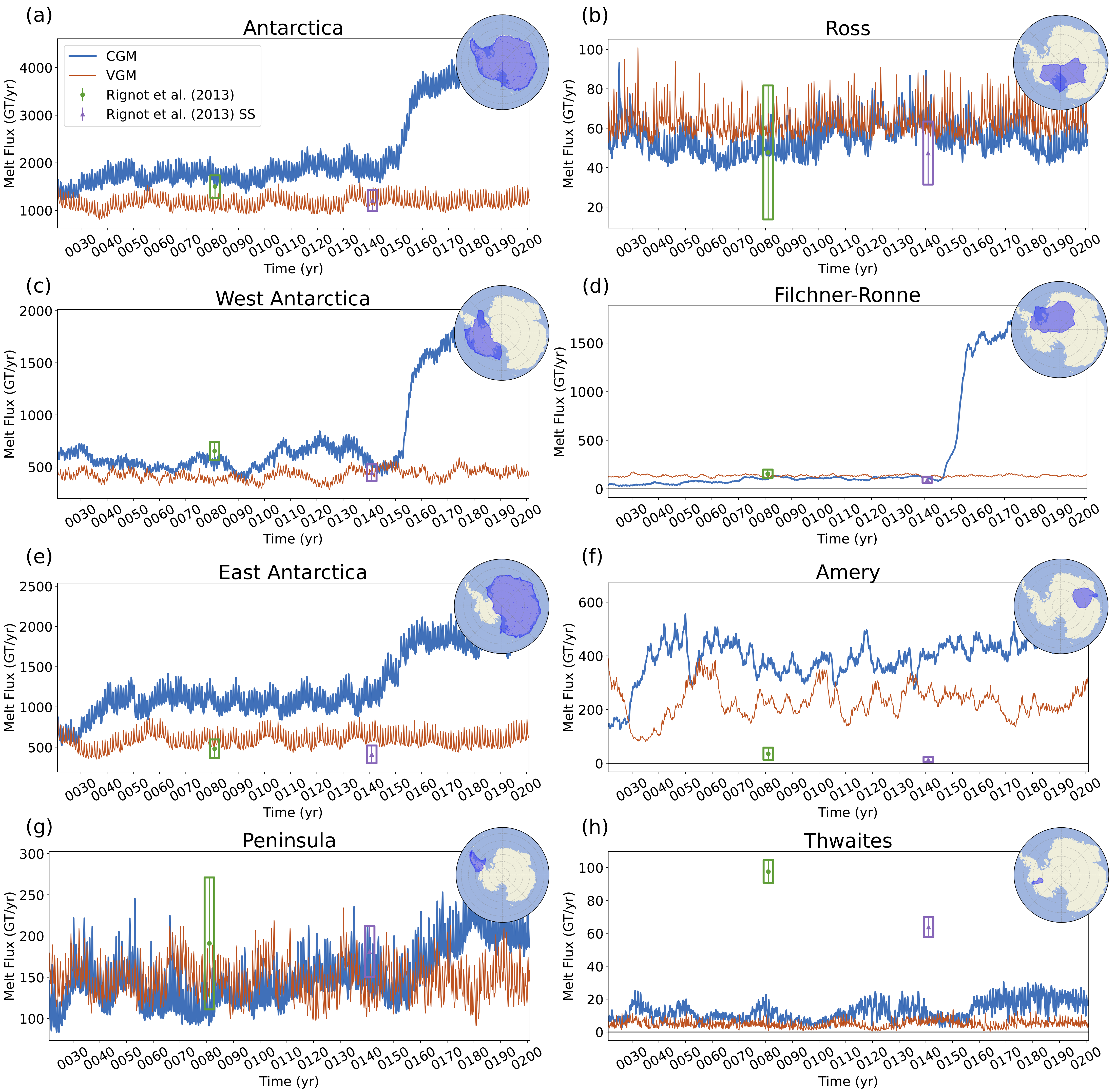
Figure 3: Time series of melt fluxes aggregated over major Antarctic regions (left) and select individual ice shelves (right) from the CGM (blue) and VGM (orange) simulations. Satellite-derived estimates for the present-day and for steady-state (i.e., assuming rates of ice-shelf thickness change are zero) melt fluxes are shown with error bars as green and purple boxes, respectively, from Rignot et al 2013; their location along the time axis is arbitrary.
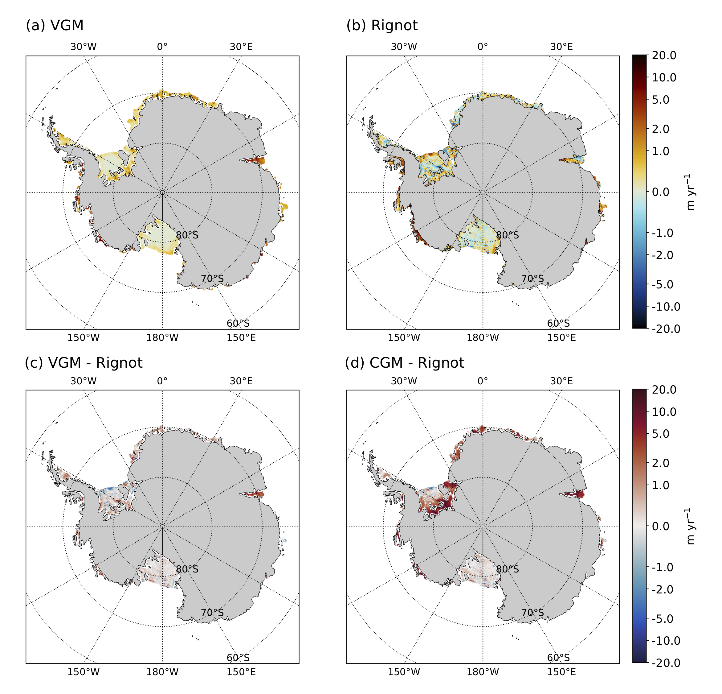
Figure 4: Map of simulated ice-shelf basal melt rates around Antarctica (a) compared to Rignot et al 2013 (b). Changes in the ocean model’s mesoscale eddy parameterization led to a drastic reduction in biases (c) vs. (d).
The simulated basal melt rates under Antarctica’s largest ice shelf, the Ross Ice Shelf, are comparable to present-day observations for both the CGM and VGM simulations. Melt rates of some small ice shelves (notably those in the Amundsen and Bellingshausen regions, e.g. Thwaites Ice Shelf in Figure 3h) are not accurately simulated in either CGM or VGM, possibly due to their poor representation at ~35 km resolution. In East Antarctica, simulated melt rates are too high relative to present-day observations in both simulations (Figure 3e), though the bias is significantly less in VGM than in CGM. The Amery Ice Shelf is the most significant contributor (Figure 3f), where again VGM simulates melt rates closer to observations, in part due to the reduced warm bias on the continental shelf relative to CGM (Figure 2e,f).
Overall, in the VGM simulation, E3SM produces realistic ice-shelf basal melt rates across the continent that are generally within the range inferred from observations (Figures 3 & 4), an important step towards reducing uncertainties in projections of the Antarctic response to earth system and Antarctica’s contribution to global sea-level change.
Publication
D. Comeau, X. Asay-Davis, C. Begeman, M. Hoffman, W. Lin, M. Petersen, S. Price, A. Roberts, L. Van Roekel, M. Veneziani, J. Wolfe, J. Fyke, T. Ringler, and A. Turner. (2020). “The DOE E3SM v1.2 Cryosphere Configuration: Description and Simulated Antarctic Ice-Shelf Basal Melting.” Journal of Advances in Modeling Earth Systems. 14, e2021MS002468. DOI: 10.1029/2021MS002468
E3SM Code
The E3SM code is available at GitHub – E3SM-Project/E3SM: Energy Exascale Earth System Model source code, and the model version used for the simulations presented here is E3SM v1.2 (Energy Exascale Earth System Model v1.2.1).
E3SM Data
The simulation data used for this paper is available on ESGF at E3SM – Home | ESGF-CoG, listed under Cryosphere-v1.2.
References
- Boyer, T. P., Garcia, H. E., Locarnini, R. A., Zweng, M. M., Mishonov, A. V., Reagan, J. R., et al. (2018). World Ocean Atlas 2018; Temperature and Salinity. NOAA Atlas NESDIS.
- Gent, P. R., & McWilliams, J. C. (1990). Isopycnal mixing in ocean circulation models. Journal of Physical Oceanography, 20(1), 150–155. https://doi.org/10.1175/1520-0485(1990)020%3C0150:IMIOCM%3E2.0.CO;2
- Rignot, E., Jacobs, S., Mouginot, J., & Scheuchl, B. (2013). Ice-shelf melting around Antarctica. Science, 341(6143), 266–270. https://doi.org/10.1126/science.1235798
- Schmidtko, S., Heywood, K. J., Thompson, A. F., & Aoki, S. (2014). Multidecadal warming of Antarctic waters. Science, 346(6214), 1227–1231. https://doi.org/10.1126/science.1256117
Funding
This research was supported as part of the Energy Exascale Earth System Model (E3SM) project, funded by the U.S. Department of Energy, Office of Science, Office of Biological and Environmental Research. This research used computing resources from the National Energy Research Scientific Computing Center (U.S. DOE contract DE-AC02-05CH11231) awarded under an ASCR Leadership Computing Challenge (ALCC) award.
Contacts
- Darin Comeau, Los Alamos National Laboratory
- Stephen Price, Los Alamos National Laboratory
- Xylar Asay-Davis, Los Alamos National Laboratory
Related Articles
This article is a part of the E3SM “Floating Points” Newsletter, to read the full Newsletter check: