

Heroic Bug Fixes: Missing Frontal Gravity Wave Correction
Bugs are an inevitable part of any complex software project, and E3SM is no exception. A lot of time goes into finding and fixing bugs, the resulting impacts can rival major parameterization changes, but these efforts and their impacts frequently go unreported. Heroic Bug Fixes is a recurring column that celebrates the critical yet often overlooked work of debugging. We hope that by shining a well-deserved spotlight on this critical work we can inspire further debugging efforts across the community and provide the broader E3SM community with timely information about changes which could aid their own development and investigations.
Gravity Waves in E3SM
Gravity waves are a ubiquitous feature of the atmosphere. Traditionally parameterized Earth system models can capture gravity waves on synoptics scales, but those on smaller scales are also critically important for large-scale circulations and need to be represented through sub-grid parameterizations. The handling of unresolved gravity wave drag (GWD) in E3SMv3 comes in three flavors: orographic, convective, and frontal. These terms describe the sources of gravity waves that the GWD schemes attempt to represent. E3SM has three GWD schemes that correspond to these sources, although they share some common infrastructure.
The GWD schemes generally take various information about unresolved processes, such as diabatic heating from the deep convection scheme, and then comes up with a spectrum of unresolved gravity waves by using various assumptions about how the sub-grid information is distributed. The schemes then make further calculations to represent how these unresolved gravity waves propagate vertically through each physics column and eventually break to deposit momentum at some level.
Similar schemes exist in other forms across various models, but the ones used in E3SM were developed many years ago at NCAR. The original schemes are associated with publications that document the methods, and while the software engineering of the schemes has been periodically updated, the underlying method has not really changed over the years.
The “frontal” GWD scheme is often not brought up in discussions of model analysis or development, partly because it is less impactful than its orographic and convective counterparts, but also because it appears to be less understood. This lack of awareness became quite problematic in the finalization of the high-resolution E3SMv3 configuration (v3HR) when a team of E3SM staff was investigating a problematic degradation of the Quasi-Biennial Oscillation (QBO) compared to the low-resolution model (v3LR).
The QBO in E3SMv3 LR vs HR
The QBO in v3LR was dramatically improved from its lackluster presence in E3SMv2. This was largely due to a new 80-layer vertical grid designed by Walter Hannah that added several layers in the lower stratosphere (see section 2.3.1 “Vertical Resolution” of the E3SMv3 Overview of the Atmospheric Component). Yu et al. (2025) showed that this modest, yet targeted, change in vertical resolution improved the ability for resolved, synoptic-scale waves to propagate upward into the stratosphere and helped to drive the QBO. At the same time, a SciDAC project led by Jim Benedict was focused on optimizing the QBO using machine learning (ML) surrogate model techniques, which help to fine-tune the QBO period to match observations. For more on these topics, see Understanding and Improving the Quasi-Biennial Oscillation in E3SM.
The success of the QBO in v3LR led many to assume that similar improvements would be evident in v3HR, but, surprisingly, this was not the case. The QBO in v3HR was much too fast, suggesting that there was way too much gravity wave forcing. Initial attempts to address this by tuning the convective GWD scheme were met with hardly any response from the model. Convective gravity waves are understood to be the dominate source of small-scale waves in the Tropics, so this is the typical way in which the QBO is tuned. This made it all the more confusing when the team found that while the low-resolution models was very sensitive to the convective GWD parameters, the high-resolution model was apparently not.
The epiphany came when the team decided to look closer at the momentum tendencies from frontal GWD scheme – which were much too large in v3HR! More thorough investigation and sensitivity analysis revealed that the frontal scheme was highly sensitive to the grid resolution, which makes all the more sense when considering the design of the scheme.
This problem was quickly alleviated by a quick adjustment of the frontal GWD scheme efficiency, which brought the QBO properties back in line with v3LR. But along the way it sparked some other curiosities about the frontal scheme, which led to a more troubling discovery.
The C&M Frontal Gravity Wave Drag Scheme
The frontal GWD scheme was introduced by Charron and Manzini (2002), and provides a framework to diagnose conditions that are favorable for frontogenesis (i.e., formation of fronts), which is most likely to occur when a strong deformation wind field acts to increase the horizontal temperature gradient (that is, the temperature varies faster across space). To this end, the “frontogenesis function” quantifies the evolution of the gradient of potential temperature (Miller 1948; Hoskins 1982; Fig. 1):
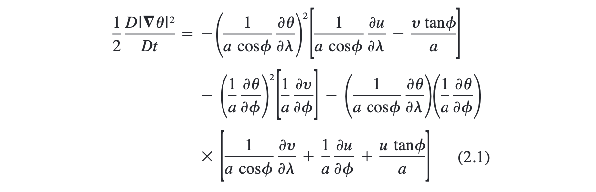
Figure 1. The frontogenesis function from Charron and Manzini (2002), which describes the evolution of the magnitude of the gradient of potential temperature (θ). The various terms describe the horizontal gradients theta along with the zonal (u) and meridional (v) wind. The horizontal gradient terms are calculated using latitude (ϕ) and longitude (λ) coordinates, where a represents the Earth’s radius.
At lower resolutions where sharp frontal boundaries cannot exist, frontogenesis is not expected to occur, but relatively large values of the frontogenesis function suggest that frontogenesis would have occurred at a sufficiently higher resolution. The frontal GWD scheme operates by calculating this quantity and comparing it to an arbitrary, tunable threshold to determine where the scheme should be active.
While this is technically accurate, the formula above assumes that the data is on surfaces of constant height, whereas E3SM uses a hybrid vertical coordinate that is not equivalent to pressure (e.g., 1000 hPa or mb) or height (e.g., 0km) coordinates. The C&M paper acknowledges this and makes note of a simple conversion to ensure that the resulting horizontal gradients are representative of geopotential height coordinates (see Fig. 2). Note that in this context the use of “altitude” or “geopotential height” are functionally equivalent, so “height” will be used to refer to the correction described in Figure 2.

Figure 2. Formula to convert gradients on model levels to gradients on constant height surfaces from Charron and Manzini (2002). In this example T represents some atmospheric scalar quantity, such as temperature, and Φ represents variable of the target vertical coordinate, such as height or geopotential. The operators ∇z and ∇𝜂 represent horizontal gradients on height and hybrid model level surfaces, respectively.
This is where the bug comes in, because while this correction may have been implemented in earlier versions of CESM – it was nowhere to be found in the active portions of CESM or E3SM in 2025! The team’s theory about how this happened is that it was lost in the switch from using the older semi-lagrangian (SL) or finite volume (FV) dynamics to the newer spectral element (SE) dynamics. Since the frontogenesis calculation relies on horizontal gradients, it is natural to utilize the gradient calculations in the model’s dynamical core (hereafter dycore), which makes the frontal GWD scheme somewhat dycore specific. An older version of the frontogenesis calculation that the team was able to locate used simple i-1 and i+1 indexing to calculate gradients. In the SE dycore, gradient calculations become much more complicated, which is likely why the gradient correction was never implemented.
What’s the Big Deal?
Why is this gradient correction term worth considering? Figure 3 below provides a demonstration of the problem it creates. In the lower free troposphere (the vertical space between the planetary boundary layer and the tropopause), where the frontogenesis calculation is assessed, the E3SM hybrid vertical coordinate is a blend of a terrain following coordinate and a pressure coordinate. This causes surfaces to be tilted relative to both height and pressure coordinates because of the underlying surface topography. This then contaminates the frontogenesis function values with stationary signals that are not indicative of potential frontogenesis.
Figure 3 is from a 1-month simulation with the default configuration of E3SMv3 (LR) and shows the frontogenesis function at the level it is evaluated for the frontal GWD scheme (the model surface nearest to 600mb). The regions indicated by red circles are areas where the influence of surface topography can clearly be seen. These signals are evident in instantaneous snapshots as well as long-term averages. These stationary signals lead to persistent activation of the frontal GWD scheme, which is clearly unphysical.
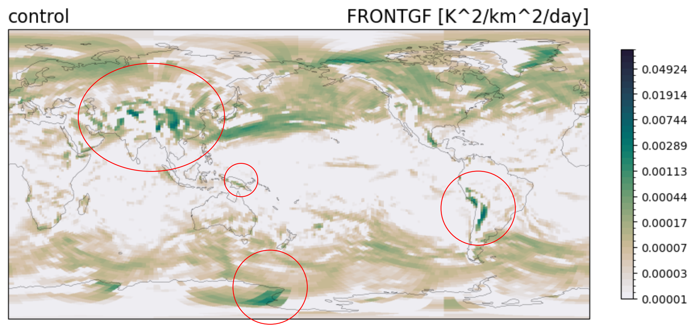
Figure 3. Frontogenesis function at the E3SMv3 (LR) vertical level closest to 600mb. Red circles indicate areas of clear influence from surface topography – the Himalayas, the Andes, the Transantarctic Mountains, and to a lesser extent in New Guinea.
Fixing the Problem
To address this problem, Walter Hannah took the initiative to implement the gradient correction term for the SE dycore. In the first version of the fix it was simpler to use a correction for constant pressure surfaces rather than height, but later the height correction was added, and both options were retained in the code.
Figure 4 shows the result of 1-month runs with either pressure and height gradient correction terms against the control. Many of the regions with notable topographic features are much less evident in the new runs, and the magnitude of frontogenesis values are generally reduced in the tropics, where frontal activity is expected to be much less than in higher latitudes.
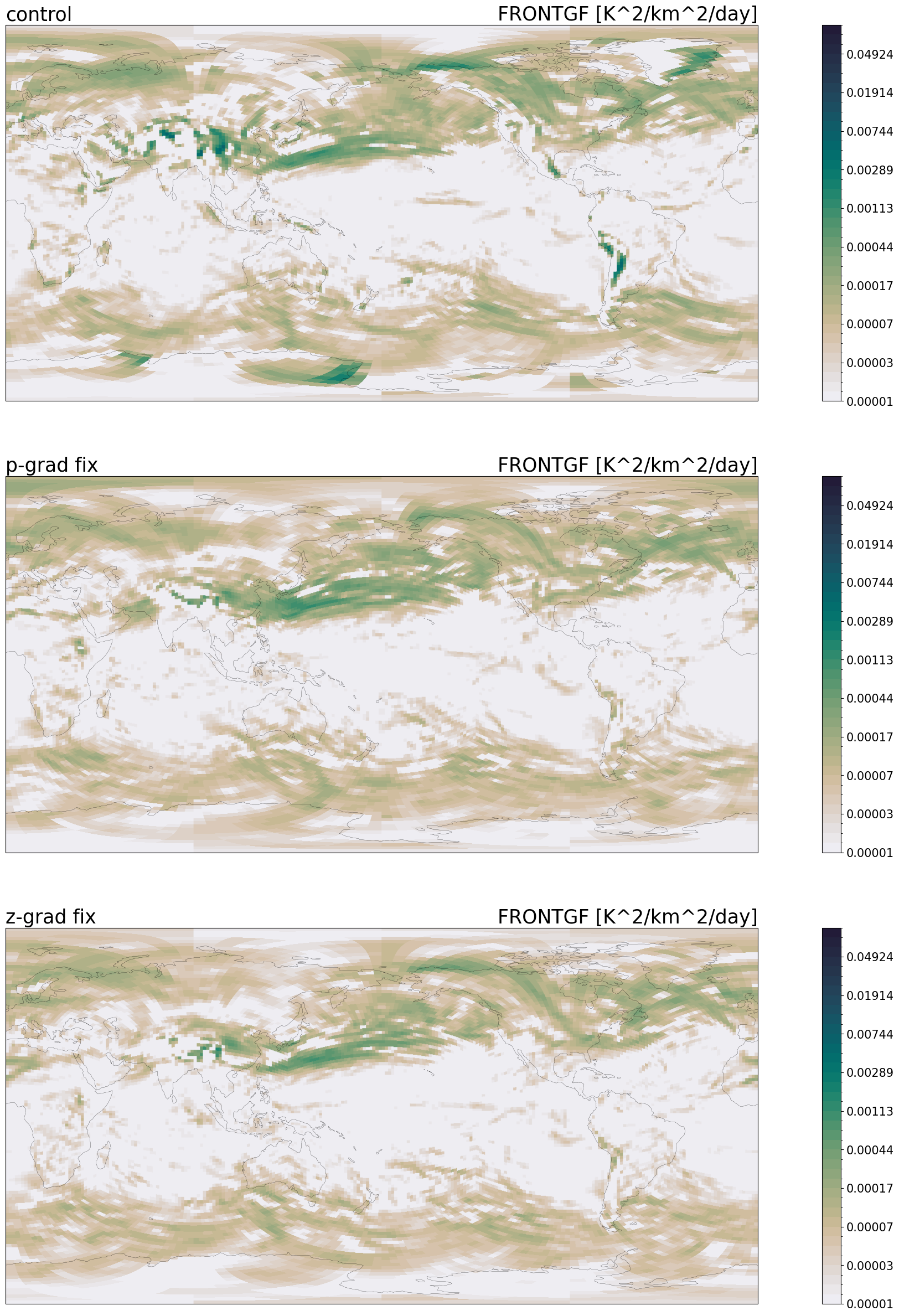
Figure 4. Frontogenesis function at the E3SMv3 (LR) vertical level closest to 600mb. The top panel, “control” is identical to Figure 3. “p-grad fix” and “z-grad fix” refer to the pressure and height gradient correction terms respectively.
Figure 5 shows the difference of both pressure and height gradient correction cases against the control to highlight that the changes are mostly taking place over areas with steep topography, as would be expected.
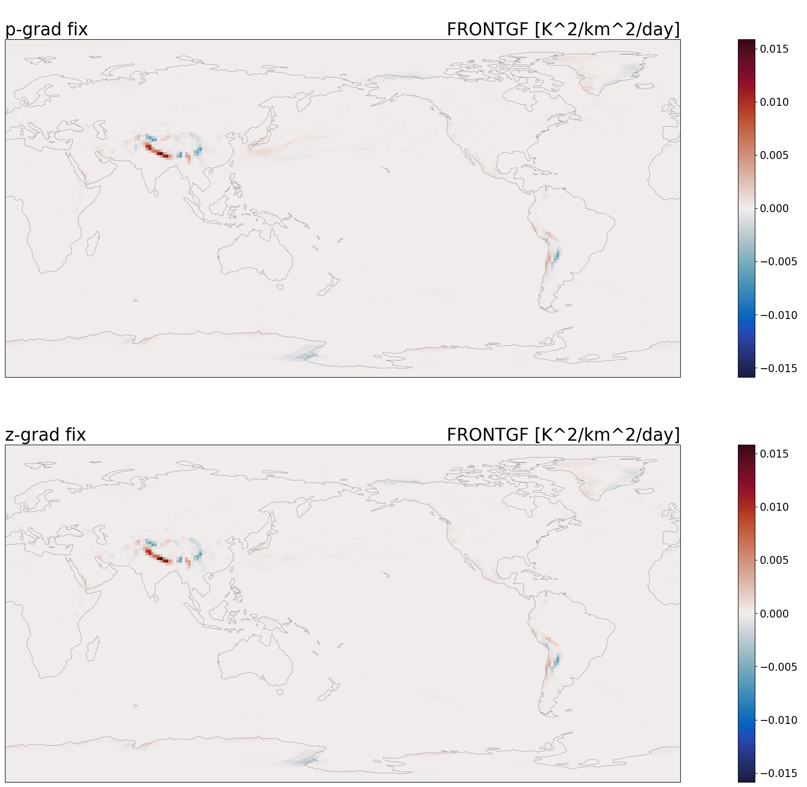
Figure 5. Frontogenesis function difference at the E3SMv3 (LR) vertical level closest to 600mb. These plots are the result of comparing the “control” run and the “fix” runs from Figure 4. Again, “p-grad fix” and “z-grad fix” refer to the pressure and height gradient correction terms respectively. Bluer colors indicate reduced frontogenesis compared to “control” while redder colors indicate increased frontogenesis.
While the correction terms have a clearly positive impact, the signals of surface topography are still evident, most notably along the Himalayas in the case with the pressure gradient correction. Figure 6 shows the height gradient correction case as a difference from the pressure gradient correction case. From this type of analysis it is not obvious that the height gradient correction approach is better, so more analysis with longer runs is likely needed to understand the tradeoffs between to the two methods. In either case, it is expected that the model will require some minor retuning of the frontal GWD parameters to adjust to the new behavior.
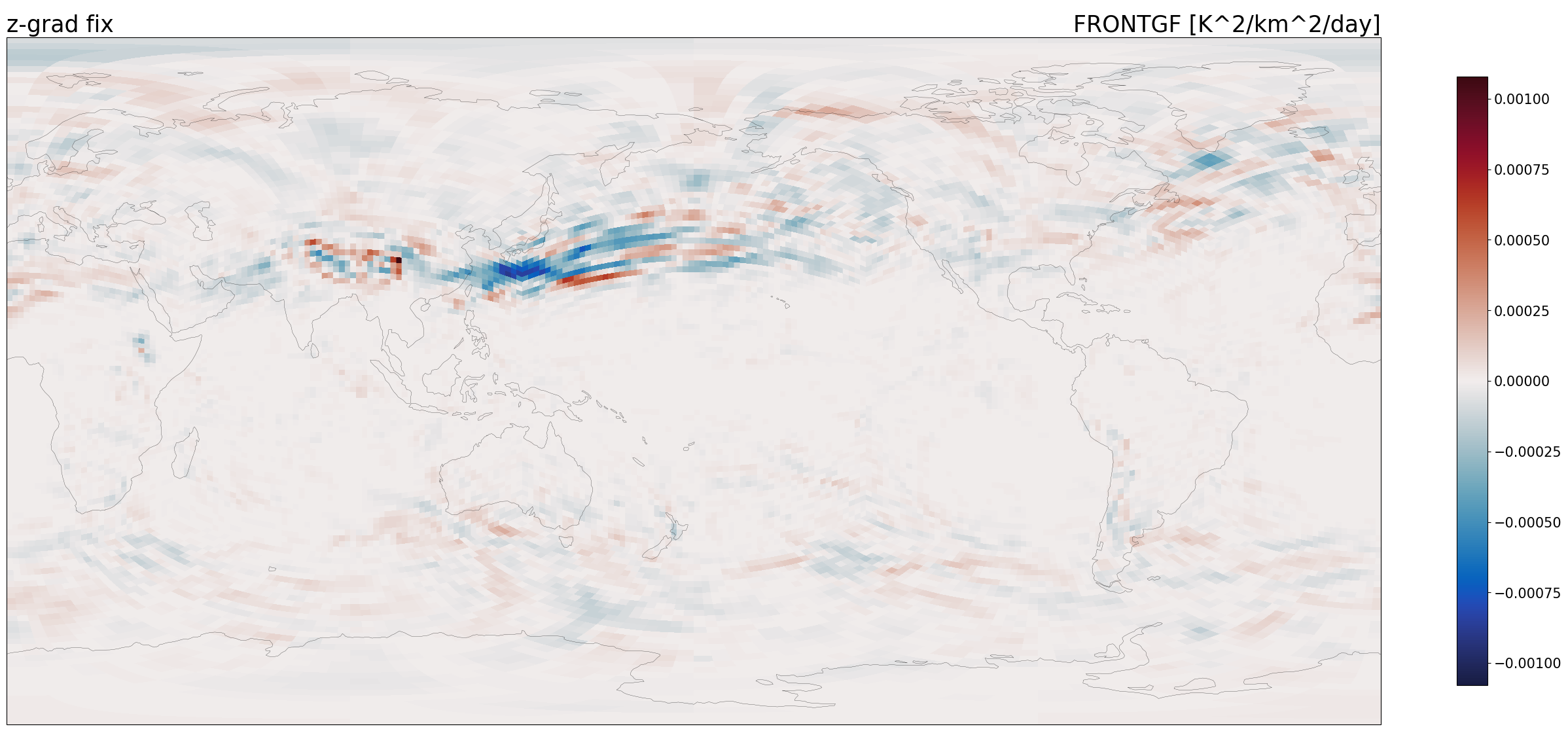
Figure 6. Frontogenesis function difference at the E3SMv3 (LR) vertical level closest to 600mb. Unlike in Figure 5, this plot was made by comparing the height gradient correction term against the pressure gradient correction term, rather than “control”. Bluer colors indicate that the height gradient correction term results in less frontogenesis than the pressure gradient correction term, whereas redder colors indicate more frontogenesis.
Unfortunately, at the time this fix was merged into E3SM both v3LR and v3HR configurations had been frozen, so the fix must be left off by default to preserve the behavior of E3SMv3. However, the team now knows the importance of carrying this new method forward for future versions.
References
- Charron, M., and E. Manzini, 2002: Gravity Waves from Fronts: Parameterization and Middle Atmosphere Response in a General Circulation Model. J. Atmos. Sci., 59, 923–941, https://doi.org/10.1175/1520-0469(2002)059%3C0923:GWFFPA%3E2.0.CO;2.
- Hoskins, B. J., 1982:: The mathematical theory of frontogenesis. Annu. Rev. Fluid Mech., 14 , 131–151.
- Miller, J. E., 1948:: On the concept of frontogenesis. J. Meteor., 5 , 169–171.
- Yu, W., Hannah, W. M., Benedict, J. J., Chen, C.-C., & Richter, J. H. (2025). Improving the QBO forcing by resolved waves with vertical grid refinement in E3SMv2. Journal of Advances in Modeling Earth Systems, 17, e2024MS004473. https://doi.org/10.1029/2024MS004473