

Representation of the Greenland Ice Sheet in E3SM

Figure 1: Greenland Ice Sheet Surface Mass Balance from low- (left) and high-resolution (center) E3SMv2 simulations with the MALI ice-sheet model. At right is Modéle Atmosphérique Régional (MAR), a regional climate model used for evaluation.
Greenland and Sea-Level Rise
The Greenland Ice Sheet (GrIS) is the primary source of freshwater from land ice that causes global sea-level rise (WCRP, 2018), with about half of its mass loss from 1992-2018 attributed to surface meltwater runoff and half to outlet glacier dynamics (Shepherd et al., 2020). The GrIS contribution to sea level is the difference between the net “surface mass balance” (SMB; the sum of mass gain through precipitation minus mass loss through sublimation and melting) and so-called “dynamic” ice sheet losses due to the flux of ice into the neighboring ocean (e.g., via iceberg calving). If outgoing flux exceeds net surface accumulation, the ice sheet loses mass and serves as a source of global sea-level rise, a situation that can occur through increased ice sheet discharge, decreased SMB, or both. Researchers estimate that GrIS SMB and ice sheet discharge were roughly in balance (at ~400 Gt/yr each) from the pre-industrial period to the mid-1990s. Since then, SMB has plummeted by about half, and discharge has increased by nearly 50%, so that the current GrIS contribution to global sea-level rise is about 1 mm/yr, and increasing. The magnitudes, relative roles, and timescales of SMB and dynamic losses to future sea-level rise are uncertain.
During E3SM Phase II, researchers from multiple institutions have been working together to improve the representation of these processes in E3SM and its component models. This includes work on E3SM’s Land Model (ELM), land ice model (MALI), and coupling infrastructure (CIME).
From Snow to Firn and Surface Mass Balance
Recent efforts to complete SMB calculations in ELM allow researchers to see how well E3SMv2 represents the GrIS SMB in near-present day (2000 CE) simulations in low and high resolution configurations (Figure 1). A defining feature of the GrIS SMB is its narrow ablation zone along its Southwest margin. Because this corridor contains a large fraction of GrIS surface melt and is central to a strong horizontal (East-West) SMB gradient, it includes processes that directly contribute to sea-level rise yet are notoriously difficult to resolve in relatively coarse resolution Earth system models (like in Low-resolution E3SMv2-LR). The GrIS has hence been the focus of recent efforts to dynamically downscale simulations of Greenland’s climate, which sharpens nominal resolution to about 25 km (Modéle Atmosphérique Régional (MAR) v3.5.2 driven by National Center for Environmental Prediction NCEPv1 reanalysis data; Fettweis et al., 2017). While refining the horizontal resolution in E3SMv2-HR improves its ability to resolve strong SMB gradients (Figure 1), future projections of the GrIS SMB require a deep snowpack (or “firn”) model that can simulate surface melt, percolation, refreezing, and retention under a rapidly warming climate.
The route to E3SM’s current, reasonable representation of GrIS SMB (Figure 1) started with the ELMv1 seasonal snowpack model, which has now been completely revamped. E3SMv1 had no active ice-sheet and its snowpack depth was limited to 1 m snow-water-equivalent (SWE). This is appropriate for modeling seasonal snowpacks but inadequate for ice sheets, which have perennial snowpacks that can exceed 100 m in thickness. The SMB that could be diagnosed from E3SMv1 was exaggerated by too quick run-off of surface melt due to the absence of pore-space for meltwater storage in the shallow snowpack, and by unrealistic snow-darkening. The “snow-capping” mass-fixer that removed water in excess of 1 m SWE from the GrIS in order to conserve water globally, also left all surface impurities (like soot) behind where they became overly concentrated and thereby unrealistically reduced albedo, further increasing melt and run-off.
To advance E3SM’s ice sheet surface processes to state of the art, its snowpack model was extended (Figure 2) to accommodate firn in Earth’s coldest regions, where substantial summer melt does not occur (Schneider et al., 2022).

Figure 2. E3SM Land Model (ELM) v1 default 5-layer vertical snowpack grid (a; 1 m) beneath which (b) the new ELMv2 firn model (activated by the “use_extrasnowlayers” namelist variable) appends up to 10 new layers that can extend as deep as 60 m, plus a bottom-most semi-infinite layer. Using 16 layers enables ELMv2 to simulate the process of firn densification and improves, relative to the CLMv5 density formulation, density profile agreement at intermediate depths with GrIS measurements (c; Mosley-Thompson et al., 2001).
On the GrIS, a massive firn layer, less dense than the ice sheet it rides on top of, can become as thick as 100 m before reaching the density at which pore space “closes off” (~830 kg/m3), entrapping air and creating bubbly ice. The duration of this entire transformation, from snow to bubbly ice, varies depending primarily on temperature and accumulation rate from snowfall, but can be longer than 1000 years. While it is a complex process to incorporate into an Earth system model, a correct density profile is critical for estimating the total pore space available for melt water retention, which buffers future sea-level rise. A more accurate GrIS firn density profile, as simulated in E3SMv2 (Figure 2c), thus marks crucial progress toward reliable projections of GrIS SMB and thus sea-level rise. The improved density profile of the ELMv2 algorithm relative to the Community Land Model (CLM) v5 algorithm (used in CESM2) at intermediate depths from 20-60 m is thought to play an important role in water storage that can help trigger ice shelf hydrofracture and eventual collapse (mainly in Antarctica) (Laffin et al., 2022).
Adding a deeper firn-snow model capable of representing GrIS SMB processes to MALI had been a long-term goal of the SciDAC4 project Probabilistic Sea Level Projections from Ice Sheet and Earth System Models (ProSPect). Concurrently, E3SM-supported UC Irvine researchers analyzed all relevant surface melt data to assess the processes that drive GrIS surface melt. Long-term measurements from the Danish Program for Monitoring of the Greenland Ice Sheet (PROMICE) Automatic Weather Station (AWS) network revealed that turbulently driven heat exchange between the surface and (usually warmer) atmosphere above plays as strong a role as solar heating in melting the ablation zone. GrIS-wide melt events produce only about 2% of surface melt (despite the anomalous attention these events receive) whereas intermittent, local, day-to-day melt associated with katabatic winds (and accompanying clear skies) produce the lion’s share of melt and run-off (Wang et al., 2021). Accounting for the observed increase of surface roughness as winds drain from the smoother accumulation zone to the rougher ablation zone is likely necessary to improve the E3SM low-resolution SMB there (compare Figure 1a vs 1b, 1c). Other key ingredients to improving GrIS SMB include properly accounting for the temperature and humidity-dependence of fresh snow grain size, and the effects of impurities on bare glacial ice albedo (Whicker et al., 2022).
Improving MPAS-Albany Land Ice (MALI) for Greenland ice sheet simulations
The spatial pattern of SMB calculated by ELM is passed through the coupler to E3SM’s land ice model, MALI, where it serves as a local mass source or sink. At each model time step, the map of SMB is used to either remove (via net melt, passed to the coupler, the runoff model, and ultimately the ocean) or add (via net accumulation) to the current ice sheet’s thickness. The ice sheet model redistributes its mass at each time step via ice flow as dictated by the momentum balance, with some ice reaching the coast and being lost to the ocean as icebergs. For the GrIS, this occurs along hundreds of marine (ocean) terminating outlet glaciers, all of which must be modeled correctly in order to make accurate projections of GrIS mass loss and sea level rise.
To this end, the ProSPect project has also been focused on adding and testing new state-of-the-art model physics and parameterizations to MALI with the goal of improving GrIS simulations in E3SM. This effort has been focused on the implementation, testing, and validation of state-of-the-art parameterizations for iceberg calving, submarine melting, and sliding at the glacier bed. The initial application of these new capabilities has been on standalone MALI simulations of Humboldt Glacier in North Greenland (Figure 3; Hillebrand et al., in review), which contains enough ice to raise global mean sea level by 19 cm and may be particularly susceptible to ocean warming (Rignot et al., 2021). For this study, we created an optimized model configuration of Humboldt Glacier for the year 2007 using observations of ice thickness, bed topography, and surface velocity. After calibrating two key model parameters to observed changes in ice extent and surface velocity from 2007–2017, we ran an ensemble of simulations to 2100, using climate forcings from three CMIP5/CMIP6 models, to constrain the range of mass loss that is consistent with observations.
All combinations of model parameters and climate forcings agree on large-scale deglaciation of the marine-based portion of Humboldt Glacier by the year 2100. We find that Humboldt is likely to contribute at least 5.5 mm to global mean sea level this century, and that it could easily contribute up to 9 mm. Compared with a recent estimate of 90±50 mm of sea-level rise from the whole Greenland Ice Sheet by 2100 (Goelzer et al., 2020), our observationally-constrained results for Humboldt Glacier represent a significant contribution from a single glacier. This could indicate that current estimates of 21st century sea-level rise from Greenland are significantly too low because whole-ice-sheet models are not generally calibrated to reproduce observed changes in historical outlet glacier velocity (and ice flux to the oceans). These new model physics and calibration methods are currently being tested for whole-ice-sheet simulations of the GrIS in E3SM, including coupling them to climate forcing from E3SM, which will lead to more realistic estimates of 21st century sea-level rise.
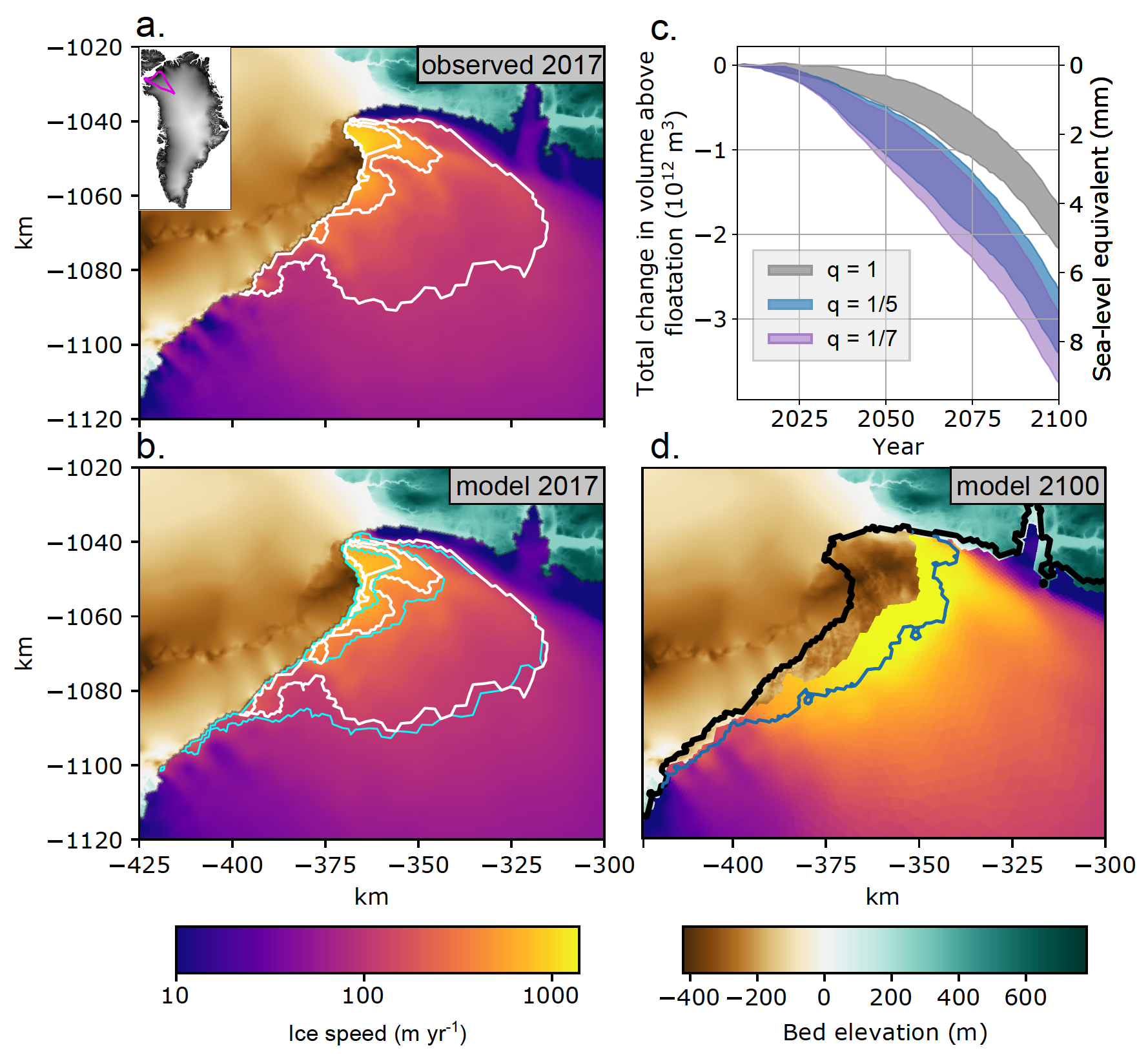
Figure 3: Demonstration of recent iceberg calving and basal sliding improvements in MALI applied to Humboldt Glacier, North Greenland (inset in (a)). Observations (a) and calibrated model (b) representation of Humboldt Glacier surface speed in 2017. Contours show speeds of 100, 300, and 600 m yr-1 from observations (white) and the model (cyan). (c) Time series of mass loss and equivalent sea-level rise (mm) from Humboldt Glacier through the 21st century when forced by three different CMIP5 and CMIP6 climate model forcings (span for each color). Different colors correspond to different treatments of basal sliding with decreasing values of “q” representing an increasingly nonlinear relationship between basal stress and sliding speed (calibrated model corresponds to q=1/5 or q=1/7). (d) Velocity snapshot at year 2100 for a single simulation. The grounding line at 2100 is shown in blue and the initial 2007 ice front in black.
Supporting a dynamic Greenland ice sheet in E3SM
In addition to the snowpack (ELM) and land ice (MALI) model improvements discussed above, infrastructure development is required to couple a dynamic GrIS model to E3SM. This includes the addition of coupler fields to pass SMB from the land model to the land ice model, routing of meltwater across and beneath the ice sheet to the ocean, and solid ice flux (from iceberg calving) to the ocean model. Additionally, appropriate compsets and grid combinations have been added to E3SM in order to allow for both “IG” (data atmosphere with active land and land ice) and “BG” (fully coupled, including active land ice) cases to be run “out-of-the-box” with a dynamic GrIS component. The first – IG cases – are useful for validation and testing of the snowpack model without incurring the cost of the fully coupled model. This capability is also important as the deeper snowpack model requires several hundred years to “spin up” and condition before it provides a realistic and dynamic SMB for use in forcing the land ice model. The second – BG cases – are the long-term target and will ultimately allow us to explore not only evolution of the GrIS but the impacts and feedbacks of a dynamic GrIS on the rest of the coupled model. This coupling work has been ongoing through E3SM Phase 1 and Phase 2, with a few key pieces yet to be completed.
Currently, E3SM supports IG and BG cases for a range of atmosphere and land resolutions (global standard and high resolutions) coupled with a variable resolution (1-to-10 km), optimized GrIS configuration for use with MALI. The variable resolution aspect is critical in order to accurately mimic dynamics within the hundreds of narrow, fast flowing marine outlets discussed above. The optimized aspect is also critical for providing both a good match between 1) the model and the present day GrIS state (the observed velocity, thickness, and ice flux) and 2) the modeled and present day ice sheet tendencies (the location and magnitude of ice thickness change). Proper optimization reduces the non-physical and unrealistic transients that result when the ice sheet model is coupled to E3SM climate forcing; unless unreasonably long and expensive coupled model spin-ups are undertaken, the climate and ice-sheet models are not in equilibrium with one another, resulting in strong coupling shocks that negate the possibility of accurate decadal-scale projections of ice-sheet mass change. The solution, being developed under the ProSPect project, is to take E3SM climate forcing into account during the GrIS model optimization process. The calibration of the ice-sheet basal friction, ice softness, and bed elevation (within observational uncertainties) is modified to include a constraint that the modeled thinning rate matches that of observations when forced by the SMB generated by E3SM. Figure 4 shows an example of the initialization of the ice sheet thermo-mechanical state for the 1-to-10 km variable resolution GrIS configuration in E3SM, where basal friction parameters have been optimized to be consistent with observations of ice sheet surface velocity.
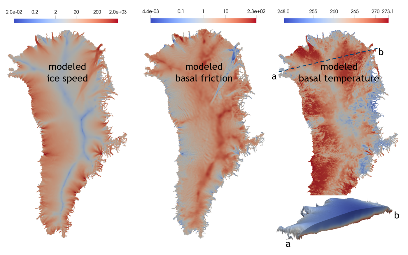
Figure 4: Ice sheet initialization obtained by optimizing the basal friction coefficient to match the observed ice surface velocity. A steady state ice temperature field is computed as part of the initialization and is self consistent with the velocity. Left: modeled velocity [m/yr]. Center: estimated basal friction [kPa yr/m]. Right: modeled steady state basal temperature [K] including a slice of vertical temperatures through the ice sheet (lower-right) along the profile line a-b.
Next Steps
To date, we have run numerous multi-decadal simulations in E3SM exercising these new capabilities. IG and BG cases have been run in order to test the new snowpack model and begin validation and SMB bias evaluation. IG and BG cases have also been run in order to confirm stable, robust (i.e., efficient and consistent land ice dycore performance), and realistic MALI evolution when forced by E3SM calculated SMB. While significant progress has been made during E3SM Phase 2, ample work remains before GrIS configurations can be considered fully supported and available for use in E3SM science applications. This additional work includes:
- extensive testing in coupled configurations (e.g., to ensure accurate and closed water budgets)
- further evaluation and improvement of SMB biases using approaches described above
- additional efforts towards coupled E3SM and ice sheet model optimization
- coupling new MALI physics (e.g., iceberg calving and frontal ablation physics, subglacial meltwater routing) with E3SM climate forcing (e.g., ocean temperature and salinity) and vice versa
- validation of coupled E3SM configurations with a dynamic GrIS against historical observations of GrIS change (with additions to E3SM-diags, MPAS-Analysis, and LIVVkit)
These improvements will enable investigations of feedbacks between glacier dynamics and SMB in Phase 3, including interactions between surface melting and basal sliding, and the impact of subglacial discharge on ocean-driven melting at marine-terminating glacier margins. The simulation of dynamic GrIS evolution in E3SM is a critical contribution to the in-progress capability of making internally consistent projections of regional sea-level change directly within E3SM.
References
Fettweis, X., Box, J. E., Agosta, C., Amory, C., Kittel, C., Lang, C., van As, D., Machguth, H., and Gallée, H. (2017). Reconstructions of the 1900–2015 Greenland ice sheet surface mass balance using the regional climate MAR model. The Cryosphere, 11, 1015–1033, https://doi.org/10.5194/tc-11-1015-2017
Goelzer, H., Nowicki, S., Payne, A., Larour, E., Seroussi, H., Lipscomb, W. H., et al. (2020). The future sea-level contribution of the Greenland ice sheet: a multi-model ensemble study of ISMIP6. The Cryosphere, 14(9), 3071–3096. https://doi.org/10.5194/tc-14-3071-2020
Hillebrand, T.R., Hoffman, M.J., Perego, M., Price, S.F., Howat, I. (2022). The contribution of Humboldt Glacier, North Greenland, to sea-level rise through 2100 constrained by recent observations of speedup and retreat. The Cryosphere (in review).
Laffin, M. K., Zender, C. S., van Wessem, J. M., and Marinsek, S. (2022). Antarctic Peninsular ice shelf collapse triggered by föhn wind-induced melt. The Cryosphere (in review).
Mosley-Thompson, E., McConnell, J. R., Bales, R. C., Li, Z., Lin, P.-N., Steffen, K., Thompson, L. G., Edwards, R., and Bathke, D. (2001), Local to regional-scale variability of annual net accumulation on the Greenland ice sheet from PARCA cores, J. Geophys. Res., 106( D24), 33839– 33851, doi:10.1029/2001JD900067
Rignot, E., An, L., Chauche, N., Morlighem, M., Jeong, S., Wood, M., et al. (2021). Retreat of Humboldt Gletscher, North Greenland, Driven by Undercutting From a Warmer Ocean. Geophysical Research Letters, 48(6), e2020GL091342. https://doi.org/10.1029/2020GL091342
Schneider, A., Zender C. S., & Price, S. (2022). More Realistic Intermediate Depth Dry Firn Densification in the Energy Exascale Earth System Model (E3SM). Journal of Advances in Modeling Earth Systems. https://doi.org/10.1029/2021MS002542
Shepherd, A. et al. (2020). Mass balance of the Greenland Ice Sheet from 1992 to 2018. Nature, 579(7798), 233–239. https://doi.org/10.1038/s41586-019-1855-2
Wang, W., Zender, C. S., van As, D., Fausto, R. S., & Laffin, M. K. (2021). Greenland surface melt dominated by solar and sensible heating. Geophysical Research Letters, 48, e2020GL090653. https://doi.org/10.1029/2020GL090653
WCRP Global Sea Level Budget Group (2018). Global sea-level budget 1993–present, Earth Syst. Sci. Data. 10, 1551–1590, https://doi.org/10.5194/essd-10-1551-2018
Whicker, C. A., Flanner, M. G., Dang, C., Zender, C. S., Cook, J. M., and Gardner, A. S. (2022): SNICAR-ADv4: A physically based radiative transfer model to represent the spectral albedo of glacier ice. The Cryosphere (in review) https://doi.org/10.5194/tc-2021-272
Funding
- Scientific Discovery through Advanced Computing (SciDAC) and Earth System Model Development (ESMD) via the Probabilistic Sea-Level Projections from Ice Sheet and Earth System Models (ProSPect) project
- This research was supported as part of the Energy Exascale Earth System Model (E3SM) project funded by the U.S. Department of Energy, Office of Science, Office of Biological and Environmental Research, through the E3SM’s sub-project “Improving Greenland ice sheet surface melt in E3SM” (LLNL-B639667).
- M. Hoffman DOE Early Career project “Creating a Sea-Level-Enabled E3SM: A Critical Capability for Predicting Coastal Impacts”
Contacts
- Charlie Zender, University of California, Irvine
- Stephen Price, Los Alamos National Laboratory
- Matt Hoffman, Los Alamos National Laboratory
Related Articles
- Projected Land Ice Contributions to 21st-Century Sea Level Rise
- Upper Bound of Antarctica’s Potential Contribution to Future Sea-Level-Rise
- Scientific Visualization of E3SM’s Cryosphere Campaign Simulations
- Antarctic Ice Sheet Modeling Highlighted on BER Website
- Antarctic Ice Shelf Collapse
- Antarctic Ocean Warming Affects Sea Level Rise
- More info on BISICLES can be found in the BISICLES Technical Highlight
- BISICLES: Adaptive Mesh Refinement for Ice Sheets
- More info on MALI can be found in the MALI Technical Highlight